Approximating Areas with Riemann Sums
Use each interval width in rectangular or trapezoidal approximations and justify any error direction.
College Board Topic 6.2 · CED p. 114 (PDF p. 119) · CED effective Fall 2020; project course outline 2026–27.
When an exact antiderivative is unavailable—or you only have samples—approximate the integral with small pieces. On [a,b], partition a = x₀ < x₁ < … < xₙ = b. A left sum uses f(xᵢ₋₁)Δxᵢ, a right sum uses f(xᵢ)Δxᵢ, and a midpoint sum uses f((xᵢ₋₁+xᵢ)/2)Δxᵢ. A trapezoid uses the average of its endpoint heights. Unequal widths are fine; calculate every width separately.
| t (min) | 0 | 1 | 3 |
|---|---|---|---|
| r(t) (L/min) | 2 | 4 | 8 |
Here left = 2(1)+4(2)=10, right = 4(1)+8(2)=20, and trapezoidal = ½(2+4)(1)+½(4+8)(2)=15 liters. For an increasing function, left underestimates and right overestimates. For a concave-up function, trapezoids overestimate and midpoint rectangles underestimate; concave down reverses that comparison. Sampled data alone do not prove behavior between samples. A calculator can add a sum or evaluate an integral, but it cannot supply a missing assumption.
Let's work through it
- Use widths 1 and 2, rather than one repeated width. Reason: The partition 0,1,3 is nonuniform.
- Add trapezoids: (2+4)/2 · 1 + (4+8)/2 · 2 = 15 L. Reason: Each trapezoid has average endpoint rate times elapsed time.
Read and estimate an increasing curved graph
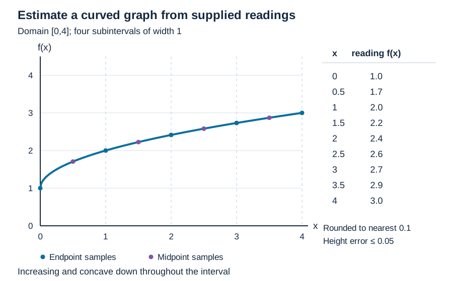
Inspect diagram labels
The diagram keeps its full size here. Focus the view and use the arrow keys, or scroll across it, to inspect every label.
Answer and check
Try it from memory
Pause & retrieve
Try it before you peek.
Write your answer and the reason from memory. Then compare with the worked answer. Your self-assessment is a study decision, not an automatically graded score.
Question 1
For decreasing f, which endpoint sum underestimates?
See every recall question with its answer
These references preserve each prompt and its answer for direct evidence links. Try the interactive questions above before opening the worked reasoning.
Retrieval 1
For decreasing f, which endpoint sum underestimates?
Worked answer and reason
The right sum.
Right endpoints give lower heights on each subinterval.
Retrieval 2
Can you compute a midpoint sum from endpoint data alone?
Worked answer and reason
Usually no.
You need values at the actual midpoints, unless an additional model is provided.
Catch the tempting mistake
- More decimal places fix an inaccurate model.
- Numerical precision and approximation error are different. Record the partition and the assumptions before rounding.
Calculator workspace and limits
For calculus, set the angle selector to Radians. This scientific calculator evaluates arithmetic and functions. It does not graph arbitrary functions, find numerical roots, evaluate numerical derivatives, or compute definite integrals. Those tasks need an approved graphing tool; the May 2027 exam permits approved handheld graphing calculators and Bluebook’s built-in Desmos on calculator-required parts. A graph or decimal estimate helps you check a conclusion; your setup, hypotheses, units and justification still do the explaining.
Scientific calculator
This calculator requires JavaScript. Use the physics formula sheets and show your working manually.
+ − * / ^ ! · pi · e · sqrt · sin, cos, tan · asin, acos, atan · atan2(y,x) · ln, log · abs · exp · hypot(x,y). Use * between factors. Keep units in your written working.
Put it to work
- Unit 6 problem 3 · No calculator · numerical
- Unit 6 problem 4 · No calculator · analytic
- Unit 6 problem 5 · No calculator · verbal
- Unit 6 problem 28 · Graphing calculator required · analytic
- Unit 6 problem 29 · No calculator · numerical
Explain and apply the mathematics
Try these problems before opening the solutions. Show your setup, the hypotheses behind your method, and what your answer means.
Estimate a supplied curved graph and qualify the result
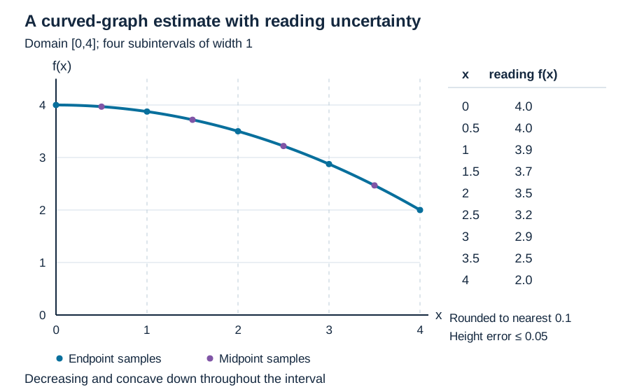
Inspect diagram labels
The diagram keeps its full size here. Focus the view and use the arrow keys, or scroll across it, to inspect every label.
Written working workspace
Drawing is temporarily unavailable. Work on paper if needed, then record your reasoning here.
Saving written working requires JavaScript. Keep your work on paper or in your own notes; the source problem above remains available.
Worked solution and rubric →Revisit the explanation →Revisit the explanation →Revisit the explanation →
Diagnose an estimate from a verbal rate description
Worked solution and rubric →Revisit the explanation →Revisit the explanation →
For the teacher
- Compare graph, formula, table, and verbal rate descriptions. Use a nonuniform table deliberately. Have students justify bounds before using the calculator.
Glossary and deeper reading · 7 refreshers
These editorial refreshers supplement the reading. Definitions and examples are added guidance; original source wording and recorded answers remain in their original context.
-
Antiderivative
An antiderivative of a function is another function whose derivative equals the original function on an interval. Two antiderivatives on the same interval differ by a constant. For example, x² is an antiderivative of 2x, and x²+7 is another. An antiderivative is a function, whereas a definite integral is an accumulated value.
-
Integral
Integration can mean accumulating a function over an interval or finding an antiderivative. A definite integral gives a number, while an indefinite integral represents a family of antiderivatives. For example, integrating 2x indefinitely gives x²+C, and integrating it from 0 to 2 gives 4. The Fundamental Theorem of Calculus connects these two operations under its hypotheses.
-
Function
A mathematical function assigns exactly one output to each input in its domain. Inputs can share an output, but one input cannot have two different outputs. For example, f(x)=x² assigns the output 9 to both 3 and −3. Function notation names the rule and its input; f(3) means the output when the input is 3.
-
Concavity
Concavity describes how a graph’s slope changes as the input increases. A graph is concave up where its derivative increases and concave down where its derivative decreases. For example, x² is concave up because its derivative 2x increases. A positive second derivative establishes concave-up behavior on an interval, while a negative one establishes concave-down behavior.
-
Continuity
A function is continuous at an input when its value exists, its finite limit exists, and those two values agree. At a domain endpoint, continuity uses the relevant one-sided approach. For example, x² is continuous at 3 because both its value and its nearby limit are 9. Continuity on an interval requires the appropriate condition at every input in that interval.
-
Definite integral
A definite integral accumulates a function over a specified interval as a limit of Riemann sums when that limit exists. Its sign includes the function’s sign and the orientation of the limits. For example, the integral of the constant −2 from 0 to 3 is −6, although the geometric area is 6. In a rate model, the result has rate units multiplied by input units.
-
Interval
An interval is a set of real numbers containing every number between any two of its members. Parentheses exclude an endpoint, while square brackets include it. For example, (1,4] includes 4 and every number between 1 and 4, but excludes 1. An infinite endpoint always uses a parenthesis because infinity is not a real endpoint.