Access this content offline
Omniguides
Skip to the reading

Interpreting the Behavior of Accumulation Functions Involving Area

Use the integrand signs and trends to analyze an accumulation function and compare its candidate values.

College Board Topic 6.5 · CED p. 117 (PDF p. 122) · CED effective Fall 2020; project course outline 2026–27.

For G(x)=∫ₐˣ f(t)dt with continuous f, G′=f and, when f is differentiable, G″=f′. So f above the axis makes G increase; f below makes G decrease. An increasing f makes G concave up; a decreasing f makes G concave down. A zero of f is a critical point of G. In the first-derivative sign test, a positive-to-negative sign change gives a local maximum and a negative-to-positive change gives a local minimum; a zero alone does not settle the question.

To find G at a point, add signed areas from the starting point; do not read the height of f as the height of G. For absolute extrema on a closed interval, compare accumulated values at endpoints and critical points. Tables of integrand values can help approximate accumulation, but signs between samples need a stated model or additional evidence.

Let's work through it

  1. Suppose f(t)=2−t and G(x)=∫₀ˣ f(t)dt on [0,4]. Then G′=2−x. Reason: Continuity permits the Fundamental Theorem.
  2. G increases up to 2 and decreases after 2, so x=2 is a maximum. Reason: G′ changes from positive to negative.
  3. G(2)=2; G(0)=G(4)=0 and G″=−1. Reason: Signed triangle area gives values; the derivative of f gives concavity.

Define the accumulation before inferring its behavior

If a continuous function f represents a signed rate, its net accumulation from a fixed reference a to a variable endpoint x is G(x) = ∫ₐˣ f(t) dt. Construct this defining integral first: the lower limit fixes the reference, the upper limit changes, and t is a dummy variable. If an amount has initial value A(a), then A(x) = A(a) + ∫ₐˣ f(t) dt. Net accumulation and total amount are different functions.

The Fundamental Theorem of Calculus gives G′(x) = f(x). Positive f makes G increase; negative f makes G decrease. A zero of f produces a horizontal tangent to G, but it is an extremum only when the sign changes. Where f increases, G is concave up; where f decreases, G is concave down. A corner of a continuous f may make G″ undefined at that point while G′ still exists. A change of concavity on the two sides can still identify an inflection point of G.

FUN-5.AFUN-5.A.2

Graphs give signs; tables need a between-sample model

For a supplied integrand graph, signed area determines the height G(x); the integrand’s height determines the slope G′(x); and the integrand’s increasing or decreasing behavior determines G’s concavity. Do not confuse a negative value of G with a negative slope. A function can remain below zero while increasing.

A raw table supplies only sampled values. Without a model, a trapezoidal sum estimates accumulation, and positive values in every row do not prove that f stays positive between rows. If linear interpolation is explicitly assumed, join adjacent rows by straight segments. Then trapezoidal areas are exact for that model, zeros can be located on each segment, and signs and concavity can be inferred from the segments. These conclusions concern the interpolation model, not every continuous function consistent with the table.

FUN-5.A.3

Carry the definition across representations

The same definition G(x) = ∫ₐˣ f(t) dt works when f is given by a graph, a numerical table with a stated model, a formula, or a verbal description. A formula may allow exact antiderivatives. A verbal statement such as “f is continuous, negative and increasing on the entire interval” determines that G decreases and is concave up, even when no exact accumulated amount is available. In every representation, use the integrand’s sign for monotonicity and its change in value for concavity.

FUN-5.A.3

Construct and analyze accumulation from a supplied graph
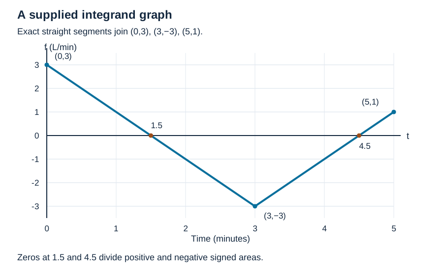
The exact continuous graph of a net inflow rate f joins (0,3), (3,−3) and (5,1) with straight segments. Time is in minutes and rate in liters per minute. A tank starts with 8 liters. Construct its net change G and amount A, then analyze G on [0,5].

The exact integrand f is made of straight segments joining (0,3), (3,−3) and (5,1). It crosses the horizontal axis at 1.5 and 4.5. Axes show t in minutes and f in liters per minute.
Exact straight segments make signed triangle and trapezoid areas available.
Inspect diagram labels

The diagram keeps its full size here. Focus the view and use the arrow keys, or scroll across it, to inspect every label.
The exact integrand f is made of straight segments joining (0,3), (3,−3) and (5,1). It crosses the horizontal axis at 1.5 and 4.5. Axes show t in minutes and f in liters per minute.

View diagram in a separate tab ↗

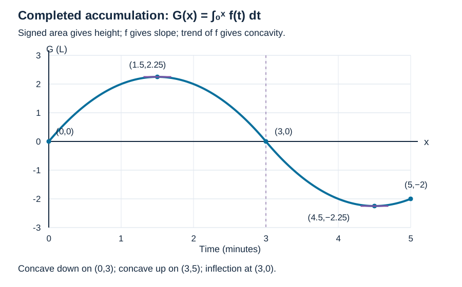
Completed graph of G(x) = integral from 0 to x of f(t) dt. It passes through (0,0), (1.5,2.25), (3,0), (4.5,−2.25) and (5,−2); it is concave down until 3 and concave up after 3.
The integrand supplies G’s slope; signed area supplies G’s height.
Inspect diagram labels

The diagram keeps its full size here. Focus the view and use the arrow keys, or scroll across it, to inspect every label.

Completed graph of G(x) = integral from 0 to x of f(t) dt. It passes through (0,0), (1.5,2.25), (3,0), (4.5,−2.25) and (5,−2); it is concave down until 3 and concave up after 3.

View diagram in a separate tab ↗

  1. The reference time is 0, so G(x) = ∫₀ˣ f(t) dt and A(x) = 8 + ∫₀ˣ f(t) dt. First construct these functions; the initial amount is not part of G.
  2. The first segment crosses zero at 1.5. Its positive triangle has area (1/2)(1.5)(3) = 2.25 liters. The next negative triangle has area −2.25, so G(1.5) = 2.25 and G(3) = 0.
  3. The second segment crosses zero at 4.5. The negative triangle from 3 to 4.5 has area −2.25, so G(4.5) = −2.25. The positive triangle from 4.5 to 5 has area (1/2)(0.5)(1) = 0.25, giving G(5) = −2 liters and A(5) = 6 liters.
  4. Because G′ = f, G increases on (0,1.5) and (4.5,5), and decreases on (1.5,4.5). Its absolute maximum is 2.25 at 1.5; its absolute minimum is −2.25 at 4.5. Endpoint values 0 and −2 do not exceed those extremes.
  5. The graph of f decreases until 3 and increases after 3. Therefore G is concave down on (0,3), concave up on (3,5), and has an inflection point at x = 3. The completed graph can be checked from G(x) = 3x − x² on [0,3] and G(x) = x² − 9x + 18 on [3,5].

Answer and check

G(x) = ∫₀ˣ f(t) dt; A(x) = 8 + G(x). G(1.5) = 2.25, G(3) = 0, G(4.5) = −2.25, G(5) = −2 liters. The integrand’s sign and trend explain the completed graph.

FUN-5.A.3

Construct an accumulation model from a nonuniform table

A continuous rate is sampled at t = 0,2,5 minutes with exact values −1,1,3 liters per minute. Assume linear interpolation between consecutive rows for this model. Construct G(x), the modeled net change since t = 0.

  1. Let f_PL be the piecewise-linear interpolation of the three rows. The requested function is G(x) = ∫₀ˣ f_PL(t) dt; this specifies which rate is being integrated.
  2. The widths are 2 and 3. Thus G(2) = 2(−1 + 1)/2 = 0 and G(5) = 0 + 3(1 + 3)/2 = 6 liters. These trapezoidal areas are exact for the stated model.
  3. The first segment crosses zero at t = 1, so G(1) = −(1/2)(1)(1) = −0.5 liters. The model is negative on (0,1) and positive on (1,5). Therefore G decreases and then increases, with absolute minimum −0.5 at 1.
  4. The modeled rate increases on both intervals, so G is concave up on (0,5). The slope of f_PL changes at 2 but does not change sign, so this is not an inflection point of G. Without linear interpolation, the table would not justify these between-row sign and concavity claims or exact areas.

Answer and check

G(x) = ∫₀ˣ f_PL(t) dt, G(1) = −0.5, G(2) = 0 and G(5) = 6 liters. Its minimum and concavity are conclusions about the stated interpolation model.

FUN-5.A.3

Construct before differentiating or interpreting

For h(t) = t² − 2t on [0,3], construct H(x), the net accumulation measured from t = 1. Separately, a continuous rate r is strictly negative and strictly increasing throughout [2,5]; construct its accumulation from 2.

  1. The defining integral for the formula is H(x) = ∫₁ˣ (t² − 2t) dt. Evaluating gives H(x) = x³/3 − x² + 2/3. In particular H(1) = 0, even though h(1) = −1.
  2. FTC gives H′(x) = h(x) = x(x − 2). Thus H decreases on (0,2) and increases on (2,3). Since h decreases on (0,1) and increases on (1,3), H is concave down and then concave up, with inflection at 1.
  3. For the verbal rate, S(x) = ∫₂ˣ r(t) dt. The stated negativity implies S(x) < 0 for x > 2 and S decreases. The stated increasing behavior of r implies S is concave up. Exact values of S cannot be computed from those qualitative facts alone.

Answer and check

H(x) = ∫₁ˣ (t² − 2t) dt = x³/3 − x² + 2/3. S(x) = ∫₂ˣ r(t) dt is negative for x > 2, decreasing and concave up under the stated whole-interval hypotheses.

FUN-5.A.3

Try it from memory

Pause & retrieve

Try it before you peek.

Write your answer and the reason from memory. Then compare with the worked answer. Your self-assessment is a study decision, not an automatically graded score.

Question 1 of 20 self-assessed

Question 1

If f is negative but increasing, how does G behave?

See every recall question with its answer

These references preserve each prompt and its answer for direct evidence links. Try the interactive questions above before opening the worked reasoning.

Retrieval 1

If f is negative but increasing, how does G behave?

Worked answer and reason

G decreases and is concave up.

The sign of f controls G′; the sign of f′ controls G″.

Retrieval 2

If f touches zero without changing sign, must G have an extremum?

Worked answer and reason

No.

An extremum requires the appropriate derivative sign change or another justification.

Catch the tempting mistake

A maximum of f is automatically a maximum of G.
A maximum of f may mark a change of concavity of G. Extrema of G come from the sign of f, not the height extrema of f.
Calculator workspace and limits

For calculus, set the angle selector to Radians. This scientific calculator evaluates arithmetic and functions. It does not graph arbitrary functions, find numerical roots, evaluate numerical derivatives, or compute definite integrals. Those tasks need an approved graphing tool; the May 2027 exam permits approved handheld graphing calculators and Bluebook’s built-in Desmos on calculator-required parts. A graph or decimal estimate helps you check a conclusion; your setup, hypotheses, units and justification still do the explaining.

Scientific calculator

This calculator requires JavaScript. Use the physics formula sheets and show your working manually.

Calculation is unavailable without JavaScript.

+ − * / ^ ! · pi · e · sqrt · sin, cos, tan · asin, acos, atan · atan2(y,x) · ln, log · abs · exp · hypot(x,y). Use * between factors. Keep units in your written working.

Put it to work

Explain and apply the mathematics

Try these problems before opening the solutions. Show your setup, the hypotheses behind your method, and what your answer means.

Build an accumulation function from an integrand graph
Calculator optional

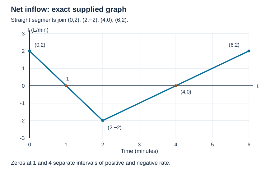
The exact graph of the continuous net inflow rate f is made of straight segments joining (0,2), (2,−2), (4,0) and (6,2), in that order. Time is measured in minutes and f in liters per minute. A tank contains 10 liters at t = 0. Define G to mean net change since time 0, and A to mean the amount in the tank.

The exact integrand f consists of straight segments joining (0,2), (2,−2), (4,0) and (6,2). Its zeros are 1 and 4. Axes show t in minutes and f in liters per minute.
The graph gives a signed net inflow rate, including negative rates.
Inspect diagram labels

The diagram keeps its full size here. Focus the view and use the arrow keys, or scroll across it, to inspect every label.

The exact integrand f consists of straight segments joining (0,2), (2,−2), (4,0) and (6,2). Its zeros are 1 and 4. Axes show t in minutes and f in liters per minute.

View diagram in a separate tab ↗

(a) Before computing areas or inferring behavior, construct defining definite-integral expressions for G(x) and A(x) for 0 ≤ x ≤ 6. Identify the reference time, the variable endpoint and the role of the initial 10 liters.

FUN-5.A

(b) Use signed areas from the supplied integrand graph to compute G(0), G(1), G(2), G(4), G(6) and A(6). State the units. Then determine the absolute maximum and minimum of G on [0,6], comparing the endpoint values as well as interior candidates.

FUN-5.A.3

(c) Using the graph of f and the Fundamental Theorem of Calculus, determine where G increases and decreases, where G is concave up and concave down, and every inflection point of G. Explain separately how the sign of f and the increasing/decreasing behavior of f lead to those conclusions. Address the corner of f at x = 2.

FUN-5.A.3FUN-5.A.2

(d) Sketch G on [0,6]. Label the five points found in part b, the horizontal tangents and the inflection point. Make your sketch agree with both the monotonicity and the concavity found in part c; explain why G can increase while its value is negative.

FUN-5.A.3

Written working workspace

Drawing is temporarily unavailable. Work on paper if needed, then record your reasoning here.

Saving written working requires JavaScript. Keep your work on paper or in your own notes; the source problem above remains available.

Written working stays in this browser.

Accumulate a nonuniform rate table under a stated model

Calculator optional

A continuous rate is sampled at the exact pairs (t,f(t)) = (0,2), (1,4), (3,−2), (4,0), with time in minutes and rate in liters per minute. For parts a–c, explicitly assume linear interpolation between each pair of consecutive rows; call that rate model f_PL. The net change is measured from time 0.

(a) Construct the defining definite integral for G(x), the accumulated net change in the piecewise-linear model, for 0 ≤ x ≤ 4. State the reference and variable endpoint. Then compute G(1), G(3) and G(4) from the nonuniform table, showing the width of each interval and explaining why trapezoidal areas are exact for this model.

FUN-5.AFUN-5.A.3LIM-5.A.2

(b) Using only the supplied table and the stated linear-interpolation model, locate each zero of f_PL. Determine where G increases and decreases, find its absolute maximum and minimum on [0,4], and determine its concavity intervals and inflection points. Show the interpolated zero calculation and the signed area needed for the interior extreme value.

FUN-5.A.3

(c) Now remove the interpolation assumption and retain only continuity and the four table rows. Decide which conclusions still hold: G′(1) = 4, the exact value G(4) = 4, increase on the whole interval (0,7/3), and concavity changes at 1 and 3. Explain what sampled values do and do not determine, and identify the status of the sum 3 + 2 − 1.

FUN-5.A.3

Written working workspace

Drawing is temporarily unavailable. Work on paper if needed, then record your reasoning here.

Saving written working requires JavaScript. Keep your work on paper or in your own notes; the source problem above remains available.

Written working stays in this browser.

Transfer accumulation reasoning to a formula and words

Calculator optional

For parts a–b, h(t) = t² − 2t on [0,3] and net accumulation is measured from t = 1. For parts c–d, r is continuous, strictly negative and strictly increasing on the entire interval [2,5]; its numerical values are not supplied.

(a) First construct H(x) as a definite integral of the supplied formula from the stated reference to x, for 0 ≤ x ≤ 3. Then obtain an explicit expression and compute H(0), H(1), H(2) and H(3). Explain why h(1) and H(1) need not be equal.

FUN-5.A

(b) From the analytic integrand h, determine where H increases and decreases, its concavity intervals, all inflection points, and its absolute maximum and minimum on [0,3]. Justify each conclusion through the integrand’s sign or trend and compare endpoints for absolute extrema.

FUN-5.A.3

(c) For the verbally described rate r, construct S(x), its net accumulation from time 2 to x, for 2 ≤ x ≤ 5. State S(2) and explain why no exact number for S(5) can be obtained from the description alone.

FUN-5.A

(d) Use the whole-interval verbal hypotheses to determine the sign of S(x) for x > 2, whether S increases or decreases, and its concavity. Explain how a negative but increasing integrand can produce the behavior you describe.

FUN-5.A.3

Written working workspace

Drawing is temporarily unavailable. Work on paper if needed, then record your reasoning here.

Saving written working requires JavaScript. Keep your work on paper or in your own notes; the source problem above remains available.

Written working stays in this browser.

Diagnose what raw rate samples establish

Calculator optional

A continuous rate f has exact samples f(0) = 2, f(1) = 4 and f(2) = 6. No interpolation, monotonicity or concavity assumption is supplied. Let G(x) = ∫₀ˣ f(t) dt.

(a) Which conclusion is justified by these hypotheses? Explain your choice using the defining integral and FTC, and identify why the other claims would need additional information between sampled times.

FUN-5.A.3

Choose your answer

Your attempt stays in this browser.

For the teacher
  • Have students annotate f with two separate marks: sign for increasing/decreasing G, and trend for concavity of G. Compare area reasoning with the analytic antiderivative.

Unit planning and formative guidance →

Glossary and deeper reading · 13 refreshers

These editorial refreshers supplement the reading. Definitions and examples are added guidance; original source wording and recorded answers remain in their original context.

  • Differentiability

    Differentiability means that a function has a finite derivative at the point under discussion. Differentiability at a point implies continuity there, but continuity alone does not imply differentiability. For example, |x| is continuous at 0 but its left and right tangent slopes differ, so it is not differentiable there. Corners, cusps, vertical tangents, and discontinuities can prevent a finite derivative.

    Read more: 2.4 · Differentiability →

  • Concavity

    Concavity describes how a graph’s slope changes as the input increases. A graph is concave up where its derivative increases and concave down where its derivative decreases. For example, x² is concave up because its derivative 2x increases. A positive second derivative establishes concave-up behavior on an interval, while a negative one establishes concave-down behavior.

    Read more: 5.6 · Concavity →

  • Absolute extremum

    An absolute extremum is the greatest or least function value on the domain or interval under discussion. The comparison includes every allowed input, including included endpoints. For example, x² on [−1,2] has absolute maximum 4 at x=2 and absolute minimum 0 at x=0. An absolute extremum must be attained rather than merely approached.

    Read more: 5.5 · Absolute extremum →

  • Interval

    An interval is a set of real numbers containing every number between any two of its members. Parentheses exclude an endpoint, while square brackets include it. For example, (1,4] includes 4 and every number between 1 and 4, but excludes 1. An infinite endpoint always uses a parenthesis because infinity is not a real endpoint.

  • Continuity

    A function is continuous at an input when its value exists, its finite limit exists, and those two values agree. At a domain endpoint, continuity uses the relevant one-sided approach. For example, x² is continuous at 3 because both its value and its nearby limit are 9. Continuity on an interval requires the appropriate condition at every input in that interval.

    Read more: 1.11 · Continuity →

  • Integral

    Integration can mean accumulating a function over an interval or finding an antiderivative. A definite integral gives a number, while an indefinite integral represents a family of antiderivatives. For example, integrating 2x indefinitely gives x²+C, and integrating it from 0 to 2 gives 4. The Fundamental Theorem of Calculus connects these two operations under its hypotheses.

    Read more: 6.7 · Integral →

  • Fundamental Theorem of Calculus

    The Fundamental Theorem of Calculus connects accumulation with differentiation. For a continuous integrand, differentiating its accumulation function returns the integrand. It also allows a definite integral of a continuous function to be evaluated by the endpoint change of an antiderivative. For example, the integral of 2x from 1 to 3 equals 3²−1²=8.

    Read more: 6.7 · Fundamental Theorem of Calculus →

  • Inflection point

    An inflection point is a point on a continuous graph where its concavity changes. A zero or undefined second derivative may identify a candidate but does not establish that change. For example, x³ changes concavity at 0, while x⁴ has second derivative zero there without changing concavity. Check the behavior on both sides of the candidate.

    Read more: 5.6 · Inflection point →

  • Integrand

    The integrand is the function or expression being integrated. The differential identifies the variable of integration. For example, in the integral of x² with respect to x, the integrand is x². Bounds belong to the integral’s interval rather than to the integrand itself.

  • Function

    A mathematical function assigns exactly one output to each input in its domain. Inputs can share an output, but one input cannot have two different outputs. For example, f(x)=x² assigns the output 9 to both 3 and −3. Function notation names the rule and its input; f(3) means the output when the input is 3.

  • Antiderivative

    An antiderivative of a function is another function whose derivative equals the original function on an interval. Two antiderivatives on the same interval differ by a constant. For example, x² is an antiderivative of 2x, and x²+7 is another. An antiderivative is a function, whereas a definite integral is an accumulated value.

    Read more: 6.8 · Antiderivative →

  • Net change

    Net change is the final amount minus the initial amount. Integrating a rate gives this signed change when the model and integral are valid. For example, moving 5 meters right and then 2 meters left gives net displacement 3 meters. Opposite contributions cancel, so net change can differ from the total amount of movement or activity.

    Read more: 8.2 · Net change →

  • Definite integral

    A definite integral accumulates a function over a specified interval as a limit of Riemann sums when that limit exists. Its sign includes the function’s sign and the orientation of the limits. For example, the integral of the constant −2 from 0 to 3 is −6, although the geometric area is 6. In a rate model, the result has rate units multiplied by input units.

    Read more: 6.3 · Definite integral →

Search lessons, terms and problems