AP Unit 7 Solutions
Worked solutions to all thirty Unit 7 problems. Each solution gives the mathematical steps and the reason for using them. Compare your setup and justification as well as the final answer.
Problem 1
A tank’s inflow is 5 L/min. Outflow is proportional to its current volume V with coefficient 0.1 min⁻¹. Write a differential equation and find the rate when V=20 L.
- Net rate is inflow minus outflow. Reason: Conservation of volume gives the derivative model.
- Substitute V=20: 5−0.1(20)=3. Reason: Evaluate the current rate from the current state.
Answer: V′=5−0.1V; rate = 3 L/min.
Final answer
V′=5−0.1V; rate = 3 L/min.
Review the teaching: Topic 7.1
Problem 2
A body’s temperature T moves toward a room temperature of 20°C at a rate proportional to the temperature difference, with positive coefficient k. Write the model and explain the sign when T=30.
- The difference from the room is T−20. Reason: The model acts on temperature difference.
- Choose −k(T−20). Reason: A body hotter than the room must cool, so the derivative is negative.
Answer: T′=−k(T−20); at T=30, T′=−10k<0.
Final answer
T′=−k(T−20); at T=30, T′=−10k<0.
Review the teaching: Topic 7.1
Problem 3
A particle’s acceleration is 2t m/s² at time t seconds, and its initial velocity is 3 m/s. Write an initial-value problem for velocity.
- Acceleration is the derivative of velocity. Reason: The motion definitions connect the two quantities.
- Record the initial velocity separately. Reason: An initial condition is a value, not an added rate.
Answer: v′(t)=2t, v(0)=3.
Final answer
v′(t)=2t, v(0)=3.
Review the teaching: Topic 7.1
Problem 4
Verify that y=3e^(2x) solves y′=2y and y(0)=3.
- Differentiate y to get y′=6e^(2x). Reason: Use the chain rule.
- Compute 2y=6e^(2x), and y(0)=3. Reason: Both sides agree throughout the domain and the initial value agrees.
Answer: It satisfies both the differential equation and initial condition for all real x.
Final answer
It satisfies both the differential equation and initial condition for all real x.
Review the teaching: Topic 7.2
Problem 5
Does y=x²+1 solve y′=2x and y(0)=0?
- Its derivative is 2x. Reason: Differentiation verifies the differential equation.
- At zero, y=1 rather than 0. Reason: Check the initial condition independently.
Answer: It solves the equation but fails the initial condition.
Final answer
It solves the equation but fails the initial condition.
Review the teaching: Topic 7.2
Problem 6
Verify that y=Ceˣ is a family of solutions to y′=y. Which member satisfies y(0)=−2?
- Differentiate Ceˣ to obtain Ceˣ=y. Reason: The equality holds for any real constant.
- Set C=y(0)=−2. Reason: The initial condition chooses this family member.
Answer: Every constant C works; the selected solution is y=−2eˣ.
Final answer
Every constant C works; the selected solution is y=−2eˣ.
Review the teaching: Topic 7.2
Problem 7
Does y=eˣ+x solve y′=y? Explain without using a graph.
- Differentiate: y′=eˣ+1, while y=eˣ+x. Reason: Verification compares the derivative to the equation’s right side.
- These agree only at x=1, not on an interval. Reason: A solution must satisfy the equation throughout its domain.
Answer: No.
Final answer
No.
Review the teaching: Topic 7.2
Problem 8
For y′=x−y, give slopes at (0,0), (1,2), and (2,−1), and describe the corresponding segments.
- Substitute each point: 0−0=0, 1−2=−1, 2−(−1)=3. Reason: A slope field evaluates the derivative at both coordinates.
- Orient short segments with those slopes. Reason: The derivative is the local tangent direction.
Answer: Slopes 0, −1, 3: horizontal, falling, and rising steeply.
Final answer
Slopes 0, −1, 3: horizontal, falling, and rising steeply.
Review the teaching: Topic 7.3
Problem 9
| y | −2 | −1 | 0 | 1 | 2 |
|---|---|---|---|---|---|
| slope | −2 | −1 | 0 | 1 | 2 |
- Slopes stay the same as x changes and match the sign and value of y. Reason: The graph and its equivalent table show slope determined by height, ruling out dependence only on x or the opposite sign.
- At y=1 the slope is positive, and positive solutions keep positive slopes. Reason: The matching equation y′=y or its verified solution y=eˣ describes the rising curve.
Answer: y′=y; the solution through (0,1) rises for increasing x.
Final answer
y′=y; the solution through (0,1) rises for increasing x.
Problem 10
For y′=x+y, where are the slope-field segments horizontal?
- Horizontal means slope zero. Reason: A horizontal tangent has derivative 0.
- Solve x+y=0 for y. Reason: The equation identifies all locations with that slope.
Answer: Along the line y=−x.
Final answer
Along the line y=−x.
Review the teaching: Topic 7.3
Problem 11
For y′=1/(x−y), can a slope-field segment be drawn at (1,1)? What is the slope at (1,0)?
- At (1,1), the denominator is zero. Reason: The differential equation is undefined there.
- At (1,0), the slope is 1/(1−0)=1. Reason: Evaluate the rule only at a defined point.
Answer: No finite segment at (1,1); slope 1 at (1,0).
Final answer
No finite segment at (1,1); slope 1 at (1,0).
Review the teaching: Topic 7.3
Problem 12
For y′=2−y, identify the equilibrium and describe a solution starting at y(0)=1 for x≥0.
- The derivative vanishes for the constant y=2; below 2 it is positive. Reason: This gives equilibrium and increasing behavior.
- Differentiate the equation: y″=−y′<0 below 2. Reason: The chain rule gives concavity.
- The solution y=2−e^(−x) confirms the forward limit 2. Reason: Solving or direct verification makes the asymptotic statement precise.
Answer: Equilibrium y=2; the solution rises toward 2 and is concave down.
Final answer
Equilibrium y=2; the solution rises toward 2 and is concave down.
Review the teaching: Topic 7.4
Problem 13
For y′=2−y, describe a solution starting at y(0)=3 for x≥0.
- Above 2, y′<0, while y″=−y′>0. Reason: The equation gives both derivative signs.
- The verified solution y=2+e^(−x) approaches 2. Reason: Its exponential term tends to zero.
Answer: It decreases toward 2 and is concave up.
Final answer
It decreases toward 2 and is concave up.
Review the teaching: Topic 7.4
Problem 14
For y′=xy, find y′ and y″ at a solution point (1,2).
- Evaluate y′=xy=2. Reason: Use the derivative rule at the specified point.
- Differentiate: y″=y+xy′=2+1·2=4. Reason: Product rule applies because y is a function of x.
Answer: y′=2 and y″=4.
Final answer
y′=2 and y″=4.
Review the teaching: Topic 7.4
Problem 15
Find the general solution of y′=2xy, including any equilibrium lost by division.
- For y≠0, separate dy/y=2x dx and integrate ln|y|=x²+C. Reason: Separation uses reverse chain-rule integration.
- Exponentiate with a signed constant A. Reason: The absolute value allows either sign.
- Check y=0 directly and include it as A=0. Reason: Division by y excluded that equilibrium.
Answer: y=Ae^(x²) for any real A, including A=0.
Final answer
y=Ae^(x²) for any real A, including A=0.
Review the teaching: Topic 7.6
Problem 16
Find the general solution of y′=x(1+y²).
- Separate dy/(1+y²)=x dx. Reason: The derivative factors into a y-dependent and an x-dependent part.
- Integrate arctan y=x²/2+C and solve for y. Reason: The arctangent derivative reverses the left side.
- Use an interval avoiding tangent poles. Reason: A solution must stay finite and differentiable.
Answer: y=tan(x²/2+C), on intervals where the tangent is defined.
Final answer
y=tan(x²/2+C), on intervals where the tangent is defined.
Review the teaching: Topic 7.6
Problem 17
Solve y′=3(1−y) generally, including its equilibrium.
- Set z=y−1; then z′=−3z. Reason: Shifting exposes a separable proportional equation.
- Integrate to z=Ae^(−3x), and restore y. Reason: Separate variables for z≠0 and include z=0 afterward.
Answer: y=1+Ae^(−3x), including A=0.
Final answer
y=1+Ae^(−3x), including A=0.
Review the teaching: Topic 7.6
Problem 18
Solve y′=xy with y(0)=2.
- Separate and integrate: y=Ae^(x²/2). Reason: The equation is separable, with the zero equilibrium included in the family.
- Apply y(0)=2 to get A=2. Reason: The initial condition selects the constant.
- Differentiate to verify y′=xy. Reason: The expression is defined and satisfies the equation for all x.
Answer: y=2e^(x²/2), all real x.
Final answer
y=2e^(x²/2), all real x.
Review the teaching: Topic 7.7
Problem 19
Solve y′=y² with y(0)=1 and give the largest interval containing 0 on which the solution is defined.
- Separate dy/y²=dx and integrate −1/y=x+C. Reason: The initial value excludes the zero equilibrium.
- Use x=0,y=1 to find C=−1; solve for y. Reason: The initial condition sets the integration constant.
- The denominator vanishes at x=1; choose the connected interval containing 0. Reason: One differentiable solution cannot pass through that singularity.
Answer: y=1/(1−x), interval (−∞,1).
Final answer
y=1/(1−x), interval (−∞,1).
Review the teaching: Topic 7.7
Problem 20
Solve y′=y/x with y(1)=3 and give a connected domain containing the initial point.
- Separate dy/y=dx/x to obtain ln|y|=ln|x|+C and y=Ax on x>0. Reason: The equation is defined only when x≠0; work on the initial point’s component.
- Use y(1)=3 to get A=3. Reason: The initial condition chooses the member.
- Restrict to (0,∞). Reason: The original equation is undefined at zero even though the formula 3x extends there.
Answer: y=3x for x>0.
Final answer
y=3x for x>0.
Review the teaching: Topic 7.7
Problem 21
Give a solution to y′=e^(−x²), y(0)=2, using an accumulation function, and verify it.
- Add the initial amount 2 to change accumulated from 0. Reason: An integral of the derivative gives net change.
- Its derivative is e^(−x²), and at x=0 the integral is zero. Reason: Continuity permits the Fundamental Theorem and verifies both requirements.
Answer: y(x)=2+∫₀ˣ e^(−t²)dt.
Final answer
y(x)=2+∫₀ˣ e^(−t²)dt.
Review the teaching: Topic 7.7
Problem 22
Solve y′=3x²−2 with y(1)=4.
- Integrate y=x³−2x+C. Reason: Reverse the derivative rules.
- Substitute 4=1−2+C, so C=5. Reason: The initial condition selects the particular solution.
Answer: y=x³−2x+5.
Final answer
y=x³−2x+5.
Review the teaching: Topic 7.7
Problem 23
Solve y′=2xy with y(0)=0.
- Test the constant zero function: its derivative and 2xy are both zero. Reason: An equilibrium can satisfy the initial condition directly.
- In the general family y=Ae^(x²), the condition gives A=0. Reason: This confirms the equilibrium is included without illegal division by zero.
Answer: y=0.
Final answer
y=0.
Review the teaching: Topic 7.7
Problem 24
Solve y′=−x/y with y(0)=2 and give the interval of this branch.
- Separate y dy=−x dx to get y²=−x²+C. Reason: The derivative is defined only for y≠0.
- Use y(0)=2 to obtain C=4 and choose the positive root. Reason: The initial condition selects both constant and branch.
- Restrict to −2<x<2. Reason: At the endpoints y=0 and the original differential equation is undefined.
Answer: y=√(4−x²), interval (−2,2).
Final answer
y=√(4−x²), interval (−2,2).
Review the teaching: Topic 7.7
Problem 25
A population follows P′=kP, P(0)=100, P(3)=200, with t in hours. Find k and P(6).
- Write P=100e^(kt); set 200=100e^(3k). Reason: Proportional growth gives the exponential family.
- Take logs for k, then evaluate at t=6. Reason: The second time interval doubles the amount again.
Answer: k=(ln2)/3 h⁻¹; P(6)=400.
Final answer
k=(ln2)/3 h⁻¹; P(6)=400.
Review the teaching: Topic 7.8
Problem 26
A substance has half-life 4 days and starts at 80 g. Give its differential equation and its amount after 12 days.
- A half-life requires e^(4k)=1/2, so k=−ln2/4 day⁻¹. Reason: Fit the exponential decay constant.
- After three half-lives, M=80(1/2)³=10 g. Reason: The model multiplies by one-half every four days.
Answer: M′=−(ln2/4)M; M(12)=10 g.
Final answer
M′=−(ln2/4)M; M(12)=10 g.
Review the teaching: Topic 7.8
Problem 27
For y′=0.05y with y(0)=100, use a calculator to find y(10) and the doubling time, to three decimals.
- Use y=100e^(0.05t), giving 100e^0.5≈164.8721271. Reason: The initial-value exponential model gives the quantity.
- Solve 2=e^(0.05T): T=ln2/0.05≈13.8629436. Reason: Doubling time follows from the ratio 2; round at the end.
Answer: y(10)≈164.872; doubling time ≈13.863 time units.
Final answer
y(10)≈164.872; doubling time ≈13.863 time units.
Review the teaching: Topic 7.8
Problem 28
A cooling model is T′=−0.2(T−20), T(0)=80, with T in °C and time in minutes. Find T(t) and its limiting temperature.
- Set D=T−20; then D′=−0.2D and D(0)=60. Reason: The temperature difference is the decaying quantity.
- Solve D=60e^(−0.2t) and add 20. Reason: Restore the original variable.
- As t→∞ the exponential tends to zero. Reason: The solution approaches the room temperature.
Answer: T(t)=20+60e^(−0.2t); limit 20°C.
Final answer
T(t)=20+60e^(−0.2t); limit 20°C.
Review the teaching: Topic 7.8
Problem 29
A particle has acceleration a(t)=2t m/s² and velocity v(0)=3 m/s. Find v(t) and its velocity at 2 s.
- Integrate v′=2t to obtain v=t²+C. Reason: Acceleration is the derivative of velocity.
- The condition gives C=3; substitute t=2. Reason: An initial velocity fixes the particular motion model.
Answer: v(t)=t²+3 m/s; v(2)=7 m/s.
Final answer
v(t)=t²+3 m/s; v(2)=7 m/s.
Review the teaching: Topic 7.8
Problem 30
A positive quantity has a continuous relative rate k=0.05 per year. Explain why its one-year percent increase is not exactly 5%, and calculate it to three decimals.
- The one-year multiplier is e^0.05. Reason: The quantity changes continuously according to y′=0.05y.
- Subtract 1 and multiply by 100 to convert relative change to percent. Reason: Interval percent change compares the final amount with the initial amount.
Answer: 100(e^0.05−1)% ≈ 5.127%.
Final answer
100(e^0.05−1)% ≈ 5.127%.
Review the teaching: Topic 7.8
Explain and apply: worked solutions
Compare the setup and the reasoning, as well as the final answer. Use the rubric to find your next step; equivalent correct reasoning earns the same credit.
Estimate two members of a solution family
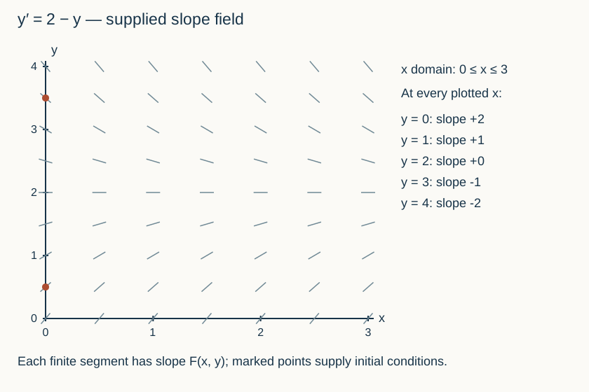
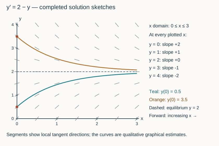
The supplied field represents y′ = 2 − y on 0 ≤ x ≤ 3 and 0 ≤ y ≤ 4. At every plotted x, slopes at y = 0, 1, 2, 3 and 4 are respectively 2, 1, 0, −1 and −2; intermediate half-unit rows follow the same rule. Two marked initial points are (0,0.5) and (0,3.5). Use qualitative graphical estimation, not a fixed-step numerical method.
Inspect diagram labels
The diagram keeps its full size here. Focus the view and use the arrow keys, or scroll across it, to inspect every label.
Inspect diagram labels
The diagram keeps its full size here. Focus the view and use the arrow keys, or scroll across it, to inspect every label.
Return to the unit problem →Try this problem in its lesson →
Follow a turning curve through a two-coordinate field
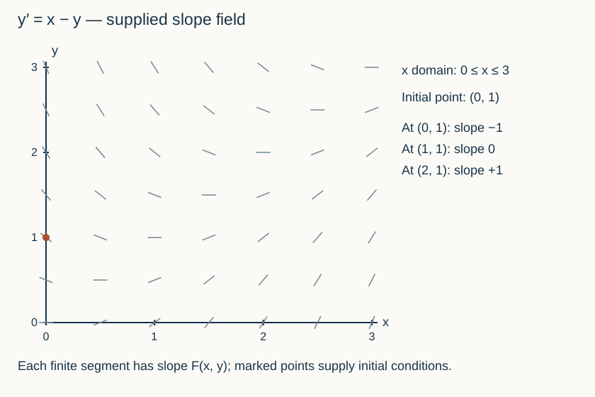
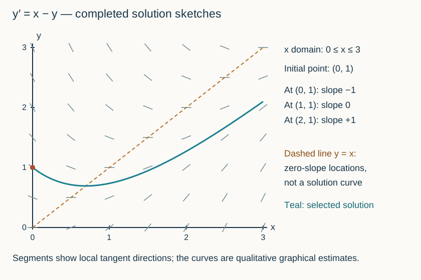
The supplied slope field represents y′ = x − y on 0 ≤ x ≤ 3 and 0 ≤ y ≤ 3. For example, slopes at (0,1), (1,1) and (2,1) are −1, 0 and +1. The selected solution passes through (0,1). Use qualitative estimation; an exact formula or numerical stepping algorithm is not required.
Inspect diagram labels
The diagram keeps its full size here. Focus the view and use the arrow keys, or scroll across it, to inspect every label.
Inspect diagram labels
The diagram keeps its full size here. Focus the view and use the arrow keys, or scroll across it, to inspect every label.
Return to the unit problem →Try this problem in its lesson →