Logistic Models with Differential Equations
Use a logistic sign chart and initial population to distinguish capacity, equilibrium, and future growth-rate behavior.
College Board Topic 7.9 · CED p. 140 (PDF p. 145) · CED effective Fall 2020; project course outline 2026–27.
BC extension: limited resources can slow proportional growth. With k>0 and carrying capacity K>0, the logistic model is P′=kP(K−P). An equivalent common form is P′=rP(1−P/K), where r=kK. The constants k and r are different: k has inverse-quantity inverse-time units, while r has inverse-time units.
Read the model without solving it. Equilibria are P=0 and P=K. If 0<P<K, the population grows; if P>K, it decreases toward K. For a positive initial population, the forward limiting value is K; an initial value of zero stays zero. The growth rate kP(K−P) is a concave-down quadratic in P, with maximum kK²/4 at P=K/2. A trajectory starting below K/2 passes through that fastest-growth level. Starting above K/2 but below K means its future growth rate decreases from the start; it does not go backward to K/2. Differentiate to see P″=kP′(K−2P), so an increasing solution changes concavity at K/2. You can reason about capacity, signs and fastest growth without a closed-form logistic solution.
Let's work through it
- For P′=0.01P(100−P), equilibria are 0 and 100. Reason: Set the derivative equal to zero.
- For P(0)=20, P′(0)=0.01·20·80=16 population units/time; the forward limit is 100. Reason: The rate is positive below capacity, and the positive solution approaches the stable equilibrium.
- The fastest growth occurs at P=50, with rate 0.01·50·50=25. Reason: The quadratic rate is maximized at half the capacity.
Two proportional factors make a product
Suppose P(t) is a population and K is its fixed carrying capacity. The statement “the net rate of change is jointly proportional to the population and its remaining capacity” names two factors: P and K − P. Joint proportionality means a constant times their product. The rate statement therefore becomes dP/dt = kP(K − P), with k > 0 for the usual growth model. The factor P represents the population available to contribute to growth. The factor K − P represents the signed shortfall from capacity: less remaining capacity reduces the net rate. Adding the factors would give P + (K − P) = K and erase this dependence on the current population.
The rate is zero at P = 0 because this model has no external source creating a population, and it is zero at P = K because the shortfall is zero. With 0 < P < K, both factors are positive. A fixed K links the factors: increasing P also decreases K − P, so doubling P alone does not generally double the full rate. For K = 1000, populations 200 and 800 give the same product, 200 × 800, even though their population sizes differ.
Use a continuous population approximation, constant positive K and k, and a time interval over which this resource model is appropriate. The usual growth domain is 0 ≤ P ≤ K. If the net-rate model is intentionally extended to P > K, the negative shortfall predicts decline; it is not a positive birth-rate law there. Negative populations have no population meaning. Changing resources, immigration or a changing K requires a reconsidered model.
The coefficient depends on the form and the units
If P and K are measured in individuals and t in days, dP/dt has units individuals/day while P(K − P) has units individuals². Therefore k has units 1/(individual·day). A measured instantaneous rate R₀ at an interior population P₀ determines k = R₀/[P₀(K − P₀)]. This calculation requires 0 < P₀ < K; an equilibrium observation gives a zero product and cannot identify k by division.
Factor K out of the shortfall: kP(K − P) = (kK)P(1 − P/K). Thus dP/dt = rP(1 − P/K), where r = kK and r has units 1/day. The remaining-capacity factor is now a dimensionless fraction, so the same numeric coefficient cannot simply be copied into both forms. At small positive P compared with K, the per-capita rate (dP/dt)/P is approximately r.
A change of population units changes k’s numerical value. If Q = P/1000 records thousands of individuals, then P = 1000Q and dP/dt = 1000 dQ/dt. Substitution gives dQ/dt = (1000k)Q(K/1000 − Q). The capacity and both population factors must use the same units. The normalized coefficient r is unchanged because r = kK = (1000k)(K/1000). The time unit is unchanged in this comparison.
Read the rate graph with the initial population
After constructing the equation, view R(P) = kP(K − P) as a graph of net rate against population. It is a downward-opening parabola with zeros 0 and K and vertex at P = K/2. Completing the square gives R(P) = kK²/4 − k(P − K/2)², so its largest positive rate is kK²/4. These axes are population and rate, not time and population.
Use the initial condition before declaring a future fastest-growth population. A trajectory with 0 < P(0) < K/2 increases through K/2 and attains that maximum rate. A trajectory starting between K/2 and K increases toward K while its rate decreases, so its greatest rate for t ≥ 0 occurs at its initial population. A positive trajectory above K decreases toward K under the extended net-rate model. For fixed positive k and K, every positive solution approaches K as t → ∞, but P(0) = 0 stays at zero. Starting at K stays at K. These conclusions use the logistic model and its initial condition without requiring a closed-form solution.
Build and calibrate a culture model
A culture is approximated continuously. Its net rate of change is jointly proportional to the number P of organisms and the number of organisms still needed to reach a fixed capacity of 1000. Time t is in hours. At P = 200 organisms, the instantaneous net increase is 32 organisms/hour. Assume constant coefficients and no external source of organisms.
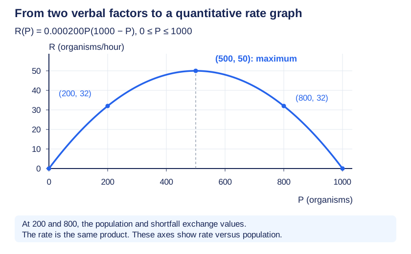
Inspect diagram labels
The diagram keeps its full size here. Focus the view and use the arrow keys, or scroll across it, to inspect every label.
- The population factor is P and the remaining-capacity factor is 1000 − P. The verbal statement therefore gives dP/dt = kP(1000 − P), with k > 0, rather than a sum or a single-factor rate.
- Calibrate at the measured interior state: 32 = k(200)(800), so k = 0.000200 1/(organism·hour). The units follow from (organisms/hour)/(organisms²).
- Rewrite as dP/dt = 0.200P(1 − P/1000). Here r = kK = 0.200/hour; it is a different coefficient with different units.
- At P = 400, the rate is 0.000200(400)(600) = 48 organisms/hour. At P = 800 it is 32 organisms/hour, equal to the rate at 200 because the two product factors exchange values.
- The rate graph has zeros 0 and 1000 and vertex at P = 500 with rate 50 organisms/hour. A trajectory starting at 200 passes through 500; one starting at 750 begins with rate 37.5 organisms/hour and thereafter has a decreasing positive rate as it approaches 1000.
Answer and check
Model: dP/dt = 0.000200P(1000 − P) = 0.200P(1 − P/1000). The 200-organism initial state grows toward capacity and reaches the rate maximum at 500; that future maximum is not reached by the 750-organism initial state.
The same lake measured in fish or thousands of fish
A lake population P is measured in fish and time in days. The net population rate is jointly proportional to P and the signed shortfall from a fixed carrying capacity of 12000 fish. At P = 3000 fish, the net increase is 270 fish/day. The constant-resource model is used with P ≥ 0. Let Q = P/1000 measure thousands of fish.
- Construct dP/dt = kP(12000 − P). From 270 = k(3000)(9000), k = 0.0000100 1/(fish·day). The normalized coefficient is r = kK = 0.120/day.
- Since P = 1000Q, dP/dt = 1000 dQ/dt and 12000 − P = 1000(12 − Q). Thus dQ/dt = 0.0100Q(12 − Q), with coefficient 0.0100 1/(thousand fish·day).
- At Q = 3, the rescaled rate is 0.0100(3)(9) = 0.270 thousand fish/day, exactly the original 270 fish/day. The coefficient increases by 1000 while the capacity decreases by 1000; their product r remains 0.120/day.
- For the dimensionless occupied fraction u = P/12000, du/dt = 0.120u(1 − u). At u = 1/4, du/dt = 0.0225/day; multiplying by 12000 fish recovers 270 fish/day.
- The three representations describe the same states and predictions when all factors, capacities and rates are converted together. Reusing 0.0000100 in the Q equation would incorrectly reduce the physical predicted rate by a factor of 1000.
Answer and check
Fish form: P′ = 0.0000100P(12000 − P). Thousands-of-fish form: Q′ = 0.0100Q(12 − Q). Fraction form: u′ = 0.120u(1 − u). The measured rate is 270 fish/day = 0.270 thousand fish/day.
Try it from memory
Pause & retrieve
Try it before you peek.
Write your answer and the reason from memory. Then compare with the worked answer. Your self-assessment is a study decision, not an automatically graded score.
Question 1
If P(0)=120 in a model with K=100, what direction does P move?
See every recall question with its answer
These references preserve each prompt and its answer for direct evidence links. Try the interactive questions above before opening the worked reasoning.
Retrieval 1
If P(0)=120 in a model with K=100, what direction does P move?
Worked answer and reason
It decreases toward 100.
The factor K−P is negative above capacity.
Retrieval 2
For P′=0.2P(1−P/500), what is the carrying capacity?
Worked answer and reason
500.
Rewrite the factor as (500−P)/500 or read where the positive equilibrium occurs.
Catch the tempting mistake
- Every logistic trajectory eventually reaches its fastest growth at K/2.
- That applies to increasing trajectories starting below K/2. If a trajectory starts between K/2 and K, its future growth rate declines; an equilibrium never grows.
Calculator workspace and limits
For calculus, set the angle selector to Radians. This scientific calculator evaluates arithmetic and functions. It does not graph arbitrary functions, find numerical roots, evaluate numerical derivatives, or compute definite integrals. Those tasks need an approved graphing tool; the May 2027 exam permits approved handheld graphing calculators and Bluebook’s built-in Desmos on calculator-required parts. A graph or decimal estimate helps you check a conclusion; your setup, hypotheses, units and justification still do the explaining.
Scientific calculator
This calculator requires JavaScript. Use the physics formula sheets and show your working manually.
+ − * / ^ ! · pi · e · sqrt · sin, cos, tan · asin, acos, atan · atan2(y,x) · ln, log · abs · exp · hypot(x,y). Use * between factors. Keep units in your written working.
Put it to work
- Unit 7 problem 28 · No calculator · verbal
- Unit 7 problem 29 · No calculator · verbal
- Unit 7 problem 30 · No calculator · verbal
Explain and apply the mathematics
Try these problems before opening the solutions. Show your setup, the hypotheses behind your method, and what your answer means.
From a verbal culture law to a rate graph
A closed culture is modeled continuously. Its net rate of change is jointly proportional to its current population and its remaining capacity. The fixed carrying capacity is 800 organisms. Let P(t) count organisms and let t be in days. When P = 200, the instantaneous net increase is 18 organisms/day. Assume a positive constant of proportionality, unchanged resources and no external source of organisms. Do not begin with a supplied differential equation.
(a) Construct the differential equation from the verbal statement using an unknown constant k. Identify and explain both factors, explain why they multiply rather than add, and give the units of k. State the ordinary growth domain and how the signed net-rate model would interpret a population above capacity.
(b) Use the measured state to determine k. Rewrite your model as rP(1 − P/800), derive the relation between r and k and give r’s units. Calculate the rates at P = 400 and P = 600. Explain why the rate at 600 can equal the measured rate at 200 even though the population is three times as large.
(c) Construct a quantitative graph of net rate R(P) versus P for 0 ≤ P ≤ 1000 using your calibrated model. Label axes and units, both zeros, the maximum, the points P = 200 and 600, and the negative-rate point at P = 900. Use the graph to determine the population and rate of greatest future growth for separate initial populations P(0) = 100 and P(0) = 600, restricting future time to t ≥ 0. Explain the distinction between a maximum of the rate law and a maximum actually visited by a trajectory.
(d) Without solving the differential equation, determine the direction of motion and the limiting population as t → ∞ for separate initial values P(0) = 0, 200, 800 and 900. Explicitly state which limiting value is an exception to the assertion that every population approaches carrying capacity, and retain the signed net-rate extension for the 900-organism case.
Written working workspace
Drawing is temporarily unavailable. Work on paper if needed, then record your reasoning here.
Saving written working requires JavaScript. Keep your work on paper or in your own notes; the source problem above remains available.
Worked solution and rubric →Revisit the explanation →Revisit the explanation →Revisit the explanation →Revisit the explanation →Revisit the explanation →
Transfer a joint rate law across units and capacity
A lake fish population has a net rate jointly proportional to its current number of fish and the signed shortfall from a fixed capacity of 10000 fish. Time is in days. At a population of 2000 fish, the instantaneous net increase is 160 fish/day. Use a continuous model with fixed positive coefficients and no migration. Later, a separate fixed-capacity trial uses a capacity of 20000 fish. It starts anew at 2000 fish; the trial does not represent an instantaneous jump in a previously fixed carrying capacity.
(a) Starting from the verbal jointly proportional description, construct the differential equation in fish units using P(t). Explain the two factors, find the proportionality constant k and its units, and write the equivalent normalized form with coefficient r and its units. State the capacity and ordinary growth domain.
(b) Let Q(t) measure the same population in thousands of fish. Construct the corresponding jointly proportional rate equation in Q and explain the meaning of its two factors. Derive the transformed coefficient and its units by substituting P = 1000Q and relating the two derivatives. Check the prediction at Q = 2, and explain which coefficient, k or r, keeps its numerical value when only population units change.
(c) For the separate 20000-fish-capacity trial, first retain the same joint proportionality coefficient k in fish units. Construct the trial’s rate equation and calculate its rate at 2000 fish and its normalized coefficient r. Contrast an alternative trial that instead retains the original normalized coefficient r. Find its k and its rate at 2000 fish. Explain why changing carrying capacity alone does not specify which coefficient should stay fixed.
Written working workspace
Drawing is temporarily unavailable. Work on paper if needed, then record your reasoning here.
Saving written working requires JavaScript. Keep your work on paper or in your own notes; the source problem above remains available.
Worked solution and rubric →Revisit the explanation →Revisit the explanation →Revisit the explanation →
One rate measurement does not identify the verbal model
In a closed group of 600 people, P(t) is the number participating, modeled continuously for 0 ≤ P ≤ 600. The net participation rate is jointly proportional to the current participating population and the number still needed to reach 600. Time is in minutes. At P = 200, the measured instantaneous rate is 12 people/minute. Coefficients are positive constants over the modeled interval.
(a) Select the rate equation consistent with the verbal jointly proportional law, the measured rate and the coefficient units. Explain why both factors must remain present and why a normalized remaining-capacity fraction requires a changed coefficient.
Worked solution and rubric →Revisit the explanation →Revisit the explanation →
For the teacher
- Use a sign chart in P rather than solving the equation first. Ask students to distinguish the two common coefficient conventions and test initial populations below, at, and above capacity.
Glossary and deeper reading · 9 refreshers
These editorial refreshers supplement the reading. Definitions and examples are added guidance; original source wording and recorded answers remain in their original context.
-
Carrying capacity
Carrying capacity is the positive equilibrium level built into a logistic growth model. In y′=ky(1−y/K) with k>0, it is K. For example, K=1000 models a population approaching 1000 when it starts between 0 and 1000. It is a modeling parameter whose interpretation depends on the situation and assumptions.
-
Concavity
Concavity describes how a graph’s slope changes as the input increases. A graph is concave up where its derivative increases and concave down where its derivative decreases. For example, x² is concave up because its derivative 2x increases. A positive second derivative establishes concave-up behavior on an interval, while a negative one establishes concave-down behavior.
-
Interval
An interval is a set of real numbers containing every number between any two of its members. Parentheses exclude an endpoint, while square brackets include it. For example, (1,4] includes 4 and every number between 1 and 4, but excludes 1. An infinite endpoint always uses a parenthesis because infinity is not a real endpoint.
-
Domain
The domain of a function is the set of inputs for which the function is defined. An expression and its context can both restrict the allowed inputs. For example, the real function f(x)=1/(x−2) has domain all real numbers except 2. For a model of elapsed time, a sensible domain may also require t≥0.
-
Instantaneous rate of change
An instantaneous rate of change is the limiting average rate around one input when that limit exists. For a differentiable function, it is its derivative at that input. For example, position s(t)=t² meters has instantaneous rate 4 meters per second at t=2 seconds. The rate’s units are output units per input unit.
-
Completing the square
Completing the square rewrites a quadratic using a squared linear expression plus a constant. For a monic quadratic x²+bx+c, add and subtract (b/2)² to obtain (x+b/2)²+c−(b/2)². For example, x²+4x+7 becomes (x+2)²+3. The rewritten form can reveal a vertex or prepare an integral for substitution.
-
Initial condition
An initial condition specifies a solution’s value at a particular input. It can determine the constant in a family of solutions to a differential equation. For example, y′=2x with y(0)=3 selects y=x²+3. The solution must satisfy both the equation and the stated condition on a suitable interval.
-
Differential equation
A differential equation relates an unknown function to one or more of its derivatives. A solution is a function that makes the equation true throughout an appropriate interval. For example, y′=2x has solutions y=x²+C. An initial condition can select a particular member of a family of solutions.
-
Derivative
A derivative gives the instantaneous rate of change of a function with respect to its input. At a point, it is the finite limit of the difference quotient when that limit exists. For example, the derivative of x² is 2x, so the tangent slope at x=3 is 6. A derivative function collects those rates across the inputs where the function is differentiable.