AP Unit 7 Solutions
Worked solutions to all thirty Unit 7 problems. Each solution gives the mathematical steps and the reason for using them. Compare your setup and justification as well as the final answer.
Problem 1
A tank’s inflow is 5 L/min. Outflow is proportional to its current volume V with coefficient 0.1 min⁻¹. Write a differential equation and find the rate when V=20 L.
- Net rate is inflow minus outflow. Reason: Conservation of volume gives the derivative model.
- Substitute V=20: 5−0.1(20)=3. Reason: Evaluate the current rate from the current state.
Answer: V′=5−0.1V; rate = 3 L/min.
Final answer
V′=5−0.1V; rate = 3 L/min.
Review the teaching: Topic 7.1
Problem 2
A body’s temperature T moves toward a room temperature of 20°C at a rate proportional to the temperature difference, with positive coefficient k. Write the model and explain the sign when T=30.
- The difference from the room is T−20. Reason: The model acts on temperature difference.
- Choose −k(T−20). Reason: A body hotter than the room must cool, so the derivative is negative.
Answer: T′=−k(T−20); at T=30, T′=−10k<0.
Final answer
T′=−k(T−20); at T=30, T′=−10k<0.
Review the teaching: Topic 7.1
Problem 3
A particle’s acceleration is 2t m/s² at time t seconds, and its initial velocity is 3 m/s. Write an initial-value problem for velocity.
- Acceleration is the derivative of velocity. Reason: The motion definitions connect the two quantities.
- Record the initial velocity separately. Reason: An initial condition is a value, not an added rate.
Answer: v′(t)=2t, v(0)=3.
Final answer
v′(t)=2t, v(0)=3.
Review the teaching: Topic 7.1
Problem 4
Verify that y=3e^(2x) solves y′=2y and y(0)=3.
- Differentiate y to get y′=6e^(2x). Reason: Use the chain rule.
- Compute 2y=6e^(2x), and y(0)=3. Reason: Both sides agree throughout the domain and the initial value agrees.
Answer: It satisfies both the differential equation and initial condition for all real x.
Final answer
It satisfies both the differential equation and initial condition for all real x.
Review the teaching: Topic 7.2
Problem 5
Does y=x²+1 solve y′=2x and y(0)=0?
- Its derivative is 2x. Reason: Differentiation verifies the differential equation.
- At zero, y=1 rather than 0. Reason: Check the initial condition independently.
Answer: It solves the equation but fails the initial condition.
Final answer
It solves the equation but fails the initial condition.
Review the teaching: Topic 7.2
Problem 6
Verify that y=Ceˣ is a family of solutions to y′=y. Which member satisfies y(0)=−2?
- Differentiate Ceˣ to obtain Ceˣ=y. Reason: The equality holds for any real constant.
- Set C=y(0)=−2. Reason: The initial condition chooses this family member.
Answer: Every constant C works; the selected solution is y=−2eˣ.
Final answer
Every constant C works; the selected solution is y=−2eˣ.
Review the teaching: Topic 7.2
Problem 7
For y′=x−y, give slopes at (0,0), (1,2), and (2,−1), and describe the corresponding segments.
- Substitute each point: 0−0=0, 1−2=−1, 2−(−1)=3. Reason: A slope field evaluates the derivative at both coordinates.
- Orient short segments with those slopes. Reason: The derivative is the local tangent direction.
Answer: Slopes 0, −1, 3: horizontal, falling, and rising steeply.
Final answer
Slopes 0, −1, 3: horizontal, falling, and rising steeply.
Review the teaching: Topic 7.3
Problem 8
| y | −2 | −1 | 0 | 1 | 2 |
|---|---|---|---|---|---|
| slope | −2 | −1 | 0 | 1 | 2 |
- Slopes stay the same as x changes and match the sign and value of y. Reason: The graph and its equivalent table show slope determined by height, ruling out dependence only on x or the opposite sign.
- At y=1 the slope is positive, and positive solutions keep positive slopes. Reason: The matching equation y′=y or its verified solution y=eˣ describes the rising curve.
Answer: y′=y; the solution through (0,1) rises for increasing x.
Final answer
y′=y; the solution through (0,1) rises for increasing x.
Problem 9
For y′=x+y, where are the slope-field segments horizontal?
- Horizontal means slope zero. Reason: A horizontal tangent has derivative 0.
- Solve x+y=0 for y. Reason: The equation identifies all locations with that slope.
Answer: Along the line y=−x.
Final answer
Along the line y=−x.
Review the teaching: Topic 7.3
Problem 10
For y′=1/(x−y), can a slope-field segment be drawn at (1,1)? What is the slope at (1,0)?
- At (1,1), the denominator is zero. Reason: The differential equation is undefined there.
- At (1,0), the slope is 1/(1−0)=1. Reason: Evaluate the rule only at a defined point.
Answer: No finite segment at (1,1); slope 1 at (1,0).
Final answer
No finite segment at (1,1); slope 1 at (1,0).
Review the teaching: Topic 7.3
Problem 11
For y′=2−y, identify the equilibrium and describe a solution starting at y(0)=1 for x≥0.
- The derivative vanishes for the constant y=2; below 2 it is positive. Reason: This gives equilibrium and increasing behavior.
- Differentiate the equation: y″=−y′<0 below 2. Reason: The chain rule gives concavity.
- The solution y=2−e^(−x) confirms the forward limit 2. Reason: Solving or direct verification makes the asymptotic statement precise.
Answer: Equilibrium y=2; the solution rises toward 2 and is concave down.
Final answer
Equilibrium y=2; the solution rises toward 2 and is concave down.
Review the teaching: Topic 7.4
Problem 12
For y′=2−y, describe a solution starting at y(0)=3 for x≥0.
- Above 2, y′<0, while y″=−y′>0. Reason: The equation gives both derivative signs.
- The verified solution y=2+e^(−x) approaches 2. Reason: Its exponential term tends to zero.
Answer: It decreases toward 2 and is concave up.
Final answer
It decreases toward 2 and is concave up.
Review the teaching: Topic 7.4
Problem 13
For y′=xy, find y′ and y″ at a solution point (1,2).
- Evaluate y′=xy=2. Reason: Use the derivative rule at the specified point.
- Differentiate: y″=y+xy′=2+1·2=4. Reason: Product rule applies because y is a function of x.
Answer: y′=2 and y″=4.
Final answer
y′=2 and y″=4.
Review the teaching: Topic 7.4
Problem 14
Find the general solution of y′=2xy, including any equilibrium lost by division.
- For y≠0, separate dy/y=2x dx and integrate ln|y|=x²+C. Reason: Separation uses reverse chain-rule integration.
- Exponentiate with a signed constant A. Reason: The absolute value allows either sign.
- Check y=0 directly and include it as A=0. Reason: Division by y excluded that equilibrium.
Answer: y=Ae^(x²) for any real A, including A=0.
Final answer
y=Ae^(x²) for any real A, including A=0.
Review the teaching: Topic 7.6
Problem 15
Find the general solution of y′=x(1+y²).
- Separate dy/(1+y²)=x dx. Reason: The derivative factors into a y-dependent and an x-dependent part.
- Integrate arctan y=x²/2+C and solve for y. Reason: The arctangent derivative reverses the left side.
- Use an interval avoiding tangent poles. Reason: A solution must stay finite and differentiable.
Answer: y=tan(x²/2+C), on intervals where the tangent is defined.
Final answer
y=tan(x²/2+C), on intervals where the tangent is defined.
Review the teaching: Topic 7.6
Problem 16
Solve y′=3(1−y) generally, including its equilibrium.
- Set z=y−1; then z′=−3z. Reason: Shifting exposes a separable proportional equation.
- Integrate to z=Ae^(−3x), and restore y. Reason: Separate variables for z≠0 and include z=0 afterward.
Answer: y=1+Ae^(−3x), including A=0.
Final answer
y=1+Ae^(−3x), including A=0.
Review the teaching: Topic 7.6
Problem 17
Solve y′=xy with y(0)=2.
- Separate and integrate: y=Ae^(x²/2). Reason: The equation is separable, with the zero equilibrium included in the family.
- Apply y(0)=2 to get A=2. Reason: The initial condition selects the constant.
- Differentiate to verify y′=xy. Reason: The expression is defined and satisfies the equation for all x.
Answer: y=2e^(x²/2), all real x.
Final answer
y=2e^(x²/2), all real x.
Review the teaching: Topic 7.7
Problem 18
Solve y′=y² with y(0)=1 and give the largest interval containing 0 on which the solution is defined.
- Separate dy/y²=dx and integrate −1/y=x+C. Reason: The initial value excludes the zero equilibrium.
- Use x=0,y=1 to find C=−1; solve for y. Reason: The initial condition sets the integration constant.
- The denominator vanishes at x=1; choose the connected interval containing 0. Reason: One differentiable solution cannot pass through that singularity.
Answer: y=1/(1−x), interval (−∞,1).
Final answer
y=1/(1−x), interval (−∞,1).
Review the teaching: Topic 7.7
Problem 19
Solve y′=y/x with y(1)=3 and give a connected domain containing the initial point.
- Separate dy/y=dx/x to obtain ln|y|=ln|x|+C and y=Ax on x>0. Reason: The equation is defined only when x≠0; work on the initial point’s component.
- Use y(1)=3 to get A=3. Reason: The initial condition chooses the member.
- Restrict to (0,∞). Reason: The original equation is undefined at zero even though the formula 3x extends there.
Answer: y=3x for x>0.
Final answer
y=3x for x>0.
Review the teaching: Topic 7.7
Problem 20
Give a solution to y′=e^(−x²), y(0)=2, using an accumulation function, and verify it.
- Add the initial amount 2 to change accumulated from 0. Reason: An integral of the derivative gives net change.
- Its derivative is e^(−x²), and at x=0 the integral is zero. Reason: Continuity permits the Fundamental Theorem and verifies both requirements.
Answer: y(x)=2+∫₀ˣ e^(−t²)dt.
Final answer
y(x)=2+∫₀ˣ e^(−t²)dt.
Review the teaching: Topic 7.7
Problem 21
Solve y′=−x/y with y(0)=2 and give the interval of this branch.
- Separate y dy=−x dx to get y²=−x²+C. Reason: The derivative is defined only for y≠0.
- Use y(0)=2 to obtain C=4 and choose the positive root. Reason: The initial condition selects both constant and branch.
- Restrict to −2<x<2. Reason: At the endpoints y=0 and the original differential equation is undefined.
Answer: y=√(4−x²), interval (−2,2).
Final answer
y=√(4−x²), interval (−2,2).
Review the teaching: Topic 7.7
Problem 22
A population follows P′=kP, P(0)=100, P(3)=200, with t in hours. Find k and P(6).
- Write P=100e^(kt); set 200=100e^(3k). Reason: Proportional growth gives the exponential family.
- Take logs for k, then evaluate at t=6. Reason: The second time interval doubles the amount again.
Answer: k=(ln2)/3 h⁻¹; P(6)=400.
Final answer
k=(ln2)/3 h⁻¹; P(6)=400.
Review the teaching: Topic 7.8
Problem 23
A substance has half-life 4 days and starts at 80 g. Give its differential equation and its amount after 12 days.
- A half-life requires e^(4k)=1/2, so k=−ln2/4 day⁻¹. Reason: Fit the exponential decay constant.
- After three half-lives, M=80(1/2)³=10 g. Reason: The model multiplies by one-half every four days.
Answer: M′=−(ln2/4)M; M(12)=10 g.
Final answer
M′=−(ln2/4)M; M(12)=10 g.
Review the teaching: Topic 7.8
Problem 24
For y′=0.05y with y(0)=100, use a calculator to find y(10) and the doubling time, to three decimals.
- Use y=100e^(0.05t), giving 100e^0.5≈164.8721271. Reason: The initial-value exponential model gives the quantity.
- Solve 2=e^(0.05T): T=ln2/0.05≈13.8629436. Reason: Doubling time follows from the ratio 2; round at the end.
Answer: y(10)≈164.872; doubling time ≈13.863 time units.
Final answer
y(10)≈164.872; doubling time ≈13.863 time units.
Review the teaching: Topic 7.8
Problem 25
Use Euler’s method for y′=y, y(0)=1, with two steps of size 0.5 to estimate y(1).
- At x=0, slope=1, so y₁=1+0.5·1=1.5 at x=0.5. Reason: Use the current point in the Euler recurrence.
- At x=0.5, slope=1.5, so y₂=1.5+0.5·1.5=2.25. Reason: Update the slope from the current estimated y.
Answer: y(1)≈2.25.
Final answer
y(1)≈2.25.
Review the teaching: Topic 7.5
Problem 26
For y′=x+y, y(1)=2, use one Euler step of size −0.2 to estimate y(0.8).
- The slope at the initial point is 1+2=3. Reason: Evaluate x+y before stepping.
- Use ynew=2+(−0.2)·3=1.4. Reason: A negative step moves backward using the same tangent-line formula.
Answer: y(0.8)≈1.4.
Final answer
y(0.8)≈1.4.
Review the teaching: Topic 7.5
Problem 27
For y′=2x, y(0)=0, use two Euler steps of size 0.5 to estimate y(1). Compare with the exact solution.
- At (0,0), slope=0, so y₁=0 at x=0.5. Reason: Use the left point’s derivative.
- Next slope=1, so y₂=0+0.5·1=0.5. Reason: Recompute the slope at x=0.5.
- Exact solution y=x² gives y(1)=1. Reason: Integrate y′=2x and apply the condition; the concave-up curve lies above these tangent steps.
Answer: Euler estimate 0.5; exact value 1; the estimate is low.
Final answer
Euler estimate 0.5; exact value 1; the estimate is low.
Review the teaching: Topic 7.5
Problem 28
A logistic population satisfies P′=0.01P(100−P), P(0)=20. Find the carrying capacity, initial rate, forward limit, and population at fastest growth.
- Zeros of the rate are 0 and 100, and the initial population is positive below 100. Reason: The model identifies capacity and an increasing trajectory toward it.
- P′(0)=0.01·20·80=16. Reason: Substitute the initial state.
- The quadratic 0.01P(100−P) is maximized at P=50, with value 25. Reason: A concave-down quadratic peaks at its vertex; this trajectory passes through 50.
Answer: Capacity and forward limit 100; initial rate 16; fastest growth at P=50 with rate 25.
Final answer
Capacity and forward limit 100; initial rate 16; fastest growth at P=50 with rate 25.
Review the teaching: Topic 7.9
Problem 29
A population follows P′=0.2P(1−P/500), P(0)=600. Find the carrying capacity, initial rate and limiting population.
- Rewrite the rate as (0.2/500)P(500−P). Reason: This matches the carrying-capacity convention kP(K−P).
- At P=600, rate=0.2·600·(1−600/500)=−24. Reason: Above capacity the rate is negative.
- The positive solution decreases toward 500. Reason: The rate sign points toward the stable positive equilibrium.
Answer: Capacity 500; initial rate −24 population units/time; forward limit 500.
Final answer
Capacity 500; initial rate −24 population units/time; forward limit 500.
Review the teaching: Topic 7.9
Problem 30
For P′=kP(K−P), with k,K>0, compare future growth-rate behavior when P(0)=K/4, P(0)=3K/4, and P(0)=0.
- For 0<P<K, P increases toward K, and R(P)=kP(K−P) has derivative k(K−2P). Reason: The population sign chart and rate derivative determine future behavior.
- A trajectory starting at K/4 passes through K/2; one starting at 3K/4 remains above K/2. Reason: An increasing trajectory does not revisit lower population values.
- P=0 makes both derivative and initial condition zero. Reason: It is an equilibrium, so its limit is zero rather than K.
Answer: At K/4, growth rate rises to a maximum at K/2 then falls; at 3K/4 it falls from the start; at 0 the solution stays zero.
Final answer
At K/4, growth rate rises to a maximum at K/2 then falls; at 3K/4 it falls from the start; at 0 the solution stays zero.
Review the teaching: Topic 7.9
Explain and apply: worked solutions
Compare the setup and the reasoning, as well as the final answer. Use the rubric to find your next step; equivalent correct reasoning earns the same credit.
From a verbal culture law to a rate graph
A closed culture is modeled continuously. Its net rate of change is jointly proportional to its current population and its remaining capacity. The fixed carrying capacity is 800 organisms. Let P(t) count organisms and let t be in days. When P = 200, the instantaneous net increase is 18 organisms/day. Assume a positive constant of proportionality, unchanged resources and no external source of organisms. Do not begin with a supplied differential equation.
Part a
Construct the differential equation from the verbal statement using an unknown constant k. Identify and explain both factors, explain why they multiply rather than add, and give the units of k. State the ordinary growth domain and how the signed net-rate model would interpret a population above capacity.
dP/dt = kP(800 − P), k > 0 with units 1/(organism·day). P is the population contributing to growth and 800 − P is the remaining-capacity shortfall. Joint proportionality gives their product. The usual growth domain is 0 ≤ P ≤ 800; an intentional extension above 800 gives negative net change.
- Name the rate as dP/dt. Translate “population” into P and “remaining capacity” into 800 − P.
- Joint proportionality means k times the product; adding gives the constant k·800 and cannot make the rate depend on both current factors.
- Rate units are organisms/day, while P(800 − P) has units organisms², so k has units 1/(organism·day).
- For 0 < P < 800 the rate is positive, at 0 and 800 it is zero, and for P > 800 the signed net-rate extension predicts decline. Negative P has no population meaning.
Scoring criteria
- 1 point: constructs dP/dt = kP(800 − P) without copying a given equation.
- 1 point: explains both named factors and joint multiplication, rather than a sum or one-factor model.
- 1 point: k > 0 and correct inverse-population inverse-time units.
- 1 point: states the nonnegative population/growth domain and qualifies above-capacity net decline.
Part b
Use the measured state to determine k. Rewrite your model as rP(1 − P/800), derive the relation between r and k and give r’s units. Calculate the rates at P = 400 and P = 600. Explain why the rate at 600 can equal the measured rate at 200 even though the population is three times as large.
k = 0.000150 1/(organism·day), r = 0.120/day. P′ = 0.000150P(800 − P) = 0.120P(1 − P/800). Rates at 400 and 600 are 24 and 18 organisms/day. At 200 and 600 the factors 200 and 600 exchange roles, leaving the same product.
- 18 = k(200)(600), so k = 18/120000 = 0.000150.
- Factor 800 from 800 − P: r = 800k = 0.120/day. The normalized remaining-capacity fraction has no units.
- At 400: 0.000150(400)(400) = 24. At 600: 0.000150(600)(200) = 18 organisms/day.
- The larger population factor is offset by the smaller shortfall. Proportionality to one factor does not mean the full rate scales with P while K is fixed.
Scoring criteria
- 1 point: correct k with units from the actual measured rate.
- 1 point: derives r = 800k and gives 0.120/day, with the complete equivalent equation.
- 1 point: both predicted rates with organism/day units.
- 1 point: product-based explanation of equal rates at 200 and 600.
Part c
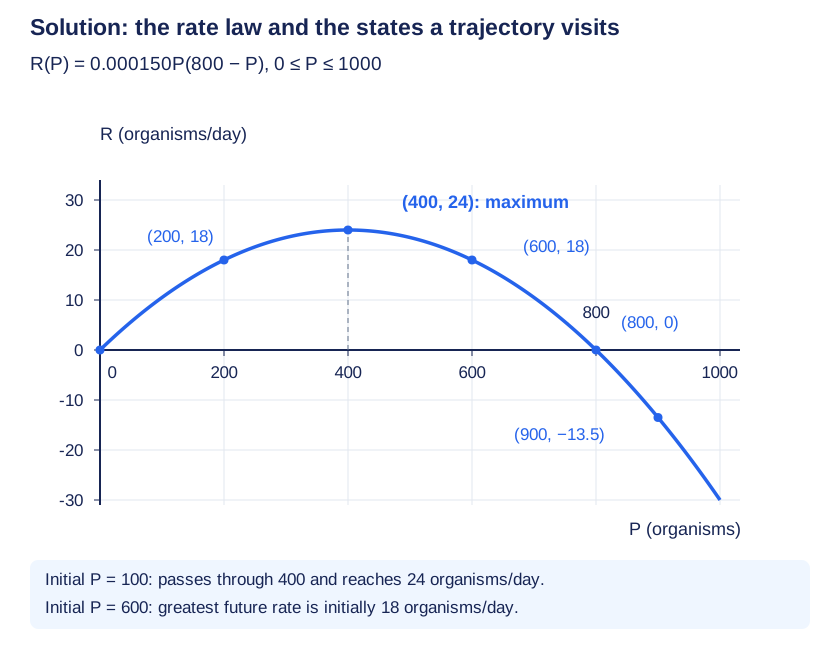
Construct a quantitative graph of net rate R(P) versus P for 0 ≤ P ≤ 1000 using your calibrated model. Label axes and units, both zeros, the maximum, the points P = 200 and 600, and the negative-rate point at P = 900. Use the graph to determine the population and rate of greatest future growth for separate initial populations P(0) = 100 and P(0) = 600, restricting future time to t ≥ 0. Explain the distinction between a maximum of the rate law and a maximum actually visited by a trajectory.
R(P) = 0.000150P(800 − P). Zeros: P = 0 and 800. Vertex: (400 organisms, 24 organisms/day). Points: (200,18), (600,18), (900,−13.5). Starting at 100, greatest future growth occurs at P = 400 with rate 24. Starting at 600, greatest future growth is initially at P = 600 with rate 18, then the positive rate decreases.
- R(P) = −0.000150P² + 0.120P is a downward-opening parabola. Its vertex is halfway between its zeros, at P = 400.
- Evaluate the displayed points and include R(900) = 0.000150(900)(−100) = −13.5 organisms/day.
- The initial 100-organism trajectory increases through 400 toward 800, so it reaches the vertex rate.
- The initial 600-organism trajectory stays between 600 and 800 for future time. On that interval the rate graph decreases with P, so the greatest future rate is its initial 18; it does not travel backward to P = 400.
Scoring criteria
- 1 point: actual downward-opening rate graph with labeled population/rate axes, units and the stated domain.
- 1 point: both zeros, vertex and all three requested nonzero points correctly plotted.
- 1 point: future maximum population/rate for initial 100 with trajectory reasoning.
- 1 point: future maximum population/rate for initial 600 and the distinction from the unattained rate-law vertex.
Part d
Without solving the differential equation, determine the direction of motion and the limiting population as t → ∞ for separate initial values P(0) = 0, 200, 800 and 900. Explicitly state which limiting value is an exception to the assertion that every population approaches carrying capacity, and retain the signed net-rate extension for the 900-organism case.
Initial 0 stays 0 and has limit 0; initial 200 increases toward 800; initial 800 stays 800; initial 900 decreases toward 800 under the stated extended net-rate model. Thus every positive initial value in this fixed logistic model has limit 800, but the zero initial value does not.
- At P = 0 or 800 one factor vanishes. These equilibrium solutions remain constant.
- On 0 < P < 800 the net rate is positive, directing a solution upward toward the stable positive equilibrium.
- On P > 800 the net rate is negative, directing the stipulated above-capacity solution downward toward 800.
- The constant-coefficient logistic model has a stable positive equilibrium at 800; positive solutions approach it. The zero solution remains the separate equilibrium and does not acquire organisms from an external source.
Scoring criteria
- 1 point: both constant equilibrium cases with their correct distinct limits.
- 1 point: initial 200 increases and tends to 800 with sign reasoning.
- 1 point: initial 900 decreases and tends to 800, explicitly within the extended net-rate model.
- 1 point: states the zero-initial exception rather than “all populations approach 800”.
Inspect diagram labels
The diagram keeps its full size here. Focus the view and use the arrow keys, or scroll across it, to inspect every label.
Return to the unit problem →Try this problem in its lesson →
Transfer a joint rate law across units and capacity
A lake fish population has a net rate jointly proportional to its current number of fish and the signed shortfall from a fixed capacity of 10000 fish. Time is in days. At a population of 2000 fish, the instantaneous net increase is 160 fish/day. Use a continuous model with fixed positive coefficients and no migration. Later, a separate fixed-capacity trial uses a capacity of 20000 fish. It starts anew at 2000 fish; the trial does not represent an instantaneous jump in a previously fixed carrying capacity.
Part a
Starting from the verbal jointly proportional description, construct the differential equation in fish units using P(t). Explain the two factors, find the proportionality constant k and its units, and write the equivalent normalized form with coefficient r and its units. State the capacity and ordinary growth domain.
P′ = kP(10000 − P), k = 0.0000100 1/(fish·day), r = 0.100/day. Equivalently P′ = 0.100P(1 − P/10000). The factors are current fish population and fish shortfall; capacity is 10000 fish and ordinary growth has 0 ≤ P ≤ 10000.
- Translate rate into P′ and the two named quantities into P and 10000 − P; joint proportionality multiplies them.
- 160 = k(2000)(8000), giving k = 0.0000100 1/(fish·day).
- Factor 10000 from the shortfall: r = kK = 0.100/day. The normalized factor is the unoccupied fraction.
- Fixed positive k/K and nonnegative populations are the model assumptions; on the usual growth interval the remaining-capacity factor is nonnegative.
Scoring criteria
- 1 point: independently constructed product model and explanation of both factors.
- 1 point: correctly calibrated k with units 1/(fish·day).
- 1 point: complete equivalent r form, derived r = kK and correct units.
- 1 point: capacity and qualified growth domain.
Part b
Let Q(t) measure the same population in thousands of fish. Construct the corresponding jointly proportional rate equation in Q and explain the meaning of its two factors. Derive the transformed coefficient and its units by substituting P = 1000Q and relating the two derivatives. Check the prediction at Q = 2, and explain which coefficient, k or r, keeps its numerical value when only population units change.
Q′ = 0.0100Q(10 − Q), where Q and 10 − Q are in thousands of fish and the coefficient is 0.0100 1/(thousand fish·day). At Q = 2 the rate is 0.160 thousand fish/day = 160 fish/day. The joint coefficient’s numeric value changes by 1000; r remains 0.100/day.
- The capacity is now 10 thousand fish, so the verbal factors become Q and 10 − Q.
- Use P′ = 1000Q′ in P′ = 0.0000100(1000Q)[1000(10 − Q)]. Divide by 1000 to obtain Q′ = 0.0100Q(10 − Q).
- At Q = 2: 0.0100(2)(8) = 0.160 thousand fish/day, matching the measured physical rate.
- The transformed capacity and coefficient satisfy (0.0100)(10) = 0.100/day. Therefore r, with inverse-time units, is unchanged while the joint coefficient changes with quantity units.
Scoring criteria
- 1 point: constructs the Q-factor and capacity-shortfall model with the converted capacity 10.
- 1 point: explicitly transforms the derivative and derives the coefficient 0.0100 with correct units.
- 1 point: checks both numerical rate and conversion to 160 fish/day.
- 1 point: explains why r is invariant while the joint coefficient’s numeric value changes.
Part c
For the separate 20000-fish-capacity trial, first retain the same joint proportionality coefficient k in fish units. Construct the trial’s rate equation and calculate its rate at 2000 fish and its normalized coefficient r. Contrast an alternative trial that instead retains the original normalized coefficient r. Find its k and its rate at 2000 fish. Explain why changing carrying capacity alone does not specify which coefficient should stay fixed.
Fixed k: P′ = 0.0000100P(20000 − P), giving 360 fish/day at P = 2000 and r = 0.200/day. Fixed r = 0.100/day: k = 0.00000500 1/(fish·day), P′ = 0.100P(1 − P/20000), giving 180 fish/day. The two assumptions preserve different physical sensitivities, so capacity change alone is insufficient.
- Fixed k gives 0.0000100(2000)(18000) = 360 fish/day and r = kK = 0.200/day.
- Fixed original r gives k = r/K = 0.100/20000 = 0.00000500 1/(fish·day), so the rate is 0.100(2000)(0.9) = 180 fish/day.
- At fixed k the proportionality between rate and the product of two count factors is retained. At fixed r the low-population per-capita coefficient is retained.
- An environmental change can affect either relation; the chosen model must state what stays fixed. Each trial treats its own capacity as constant in time.
Scoring criteria
- 1 point: correct fixed-k trial equation, 360 fish/day and r = 0.200/day.
- 1 point: correct fixed-r coefficient/equation and 180 fish/day.
- 1 point: explains the distinct held quantities and why a capacity change alone cannot choose between the models.
Return to the unit problem →Try this problem in its lesson →
One rate measurement does not identify the verbal model
In a closed group of 600 people, P(t) is the number participating, modeled continuously for 0 ≤ P ≤ 600. The net participation rate is jointly proportional to the current participating population and the number still needed to reach 600. Time is in minutes. At P = 200, the measured instantaneous rate is 12 people/minute. Coefficients are positive constants over the modeled interval.
Part a
Select the rate equation consistent with the verbal jointly proportional law, the measured rate and the coefficient units. Explain why both factors must remain present and why a normalized remaining-capacity fraction requires a changed coefficient.
P′ = 0.000150P(600 − P). The factors are the existing population P and its remaining capacity 600 − P. k = 0.000150 1/(person·minute), whereas the equivalent normalized coefficient is r = kK = 0.0900/minute.
- Translate joint proportionality into kP(600 − P). At P = 200 the product is 80000 persons², so k = 12/80000 = 0.000150 1/(person·minute).
- The correct choice gives 12 persons/minute at 200 and zero at both 0 and 600. A single-factor alternative can fit one data point yet fail the joint verbal law.
- Factoring 600 gives r = 600k = 0.0900/minute; using the original numeric k with 1 − P/600 yields only 0.0200 persons/minute if treated as an inverse-time coefficient.
Scoring criteria
- 1 point: selects the correct jointly proportional product model.
- 1 point: explains both factors and why the normalized coefficient is 600k rather than k.
Return to the unit problem →Try this problem in its lesson →
Estimate two members of a solution family
The supplied field represents y′ = 2 − y on 0 ≤ x ≤ 3 and 0 ≤ y ≤ 4. At every plotted x, slopes at y = 0, 1, 2, 3 and 4 are respectively 2, 1, 0, −1 and −2; intermediate half-unit rows follow the same rule. Two marked initial points are (0,0.5) and (0,3.5). Use qualitative graphical estimation, not a fixed-step numerical method.
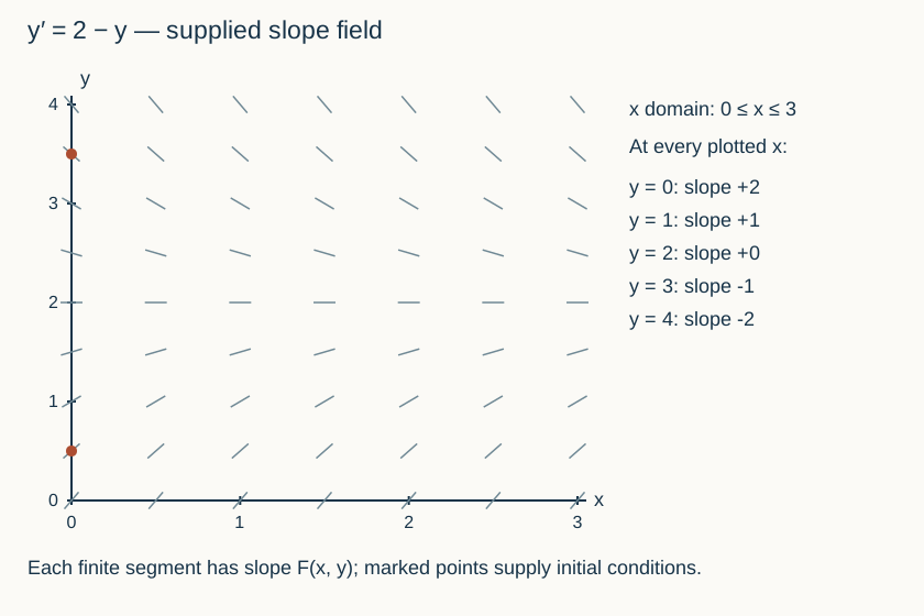
Inspect diagram labels
The diagram keeps its full size here. Focus the view and use the arrow keys, or scroll across it, to inspect every label.
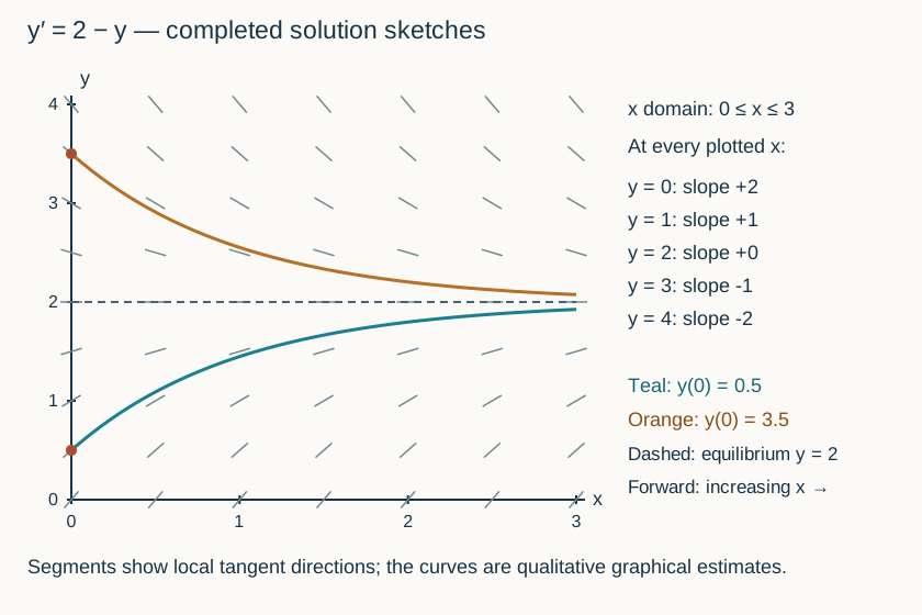
Inspect diagram labels
The diagram keeps its full size here. Focus the view and use the arrow keys, or scroll across it, to inspect every label.
Return to the unit problem →Try this problem in its lesson →
Follow a turning curve through a two-coordinate field
The supplied slope field represents y′ = x − y on 0 ≤ x ≤ 3 and 0 ≤ y ≤ 3. For example, slopes at (0,1), (1,1) and (2,1) are −1, 0 and +1. The selected solution passes through (0,1). Use qualitative estimation; an exact formula or numerical stepping algorithm is not required.
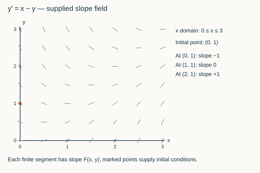
Inspect diagram labels
The diagram keeps its full size here. Focus the view and use the arrow keys, or scroll across it, to inspect every label.
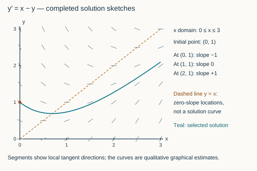
Inspect diagram labels
The diagram keeps its full size here. Focus the view and use the arrow keys, or scroll across it, to inspect every label.
Return to the unit problem →Try this problem in its lesson →