Thirty problems for AP Unit 6. Try the problem before opening its separate solution. Write the mathematical setup and the reason your method applies.
This BC unit uses shared AB problems where the content is the same, with BC extensions where needed. Reused problems keep a link to their AB source and count once in the distinct assessment inventory.
Choose your next practice
Find the problems you need.
Mix the choices to focus your practice. Problem numbers and worked-solution links stay the same.
30 of 30 problems shown.
Selection: All topics and practice types.
Printing includes the currently visible selection. Reset filters first to print all 30 problems.
Worked-example retrieval. Reconstruct the lesson reasoning before checking the solution.
Blue is positive change; orange is negative change. The text description carries the same numerical information.A velocity graph (m/s) is a triangle above the time axis on [0,2] with height 3, then a triangle below on [2,4] with depth 2. Find displacement and total distance.
Use the partition 0,2,5 to calculate the left, right, and trapezoidal approximations to ∫₀⁵ f(x)dx. Explain why averaging the three samples and multiplying by 5 is not the trapezoidal rule.
Try these problems before opening the solutions. Show your setup, the hypotheses behind your method, and what your answer means.
Estimate a supplied curved graph and qualify the result
Calculator optional
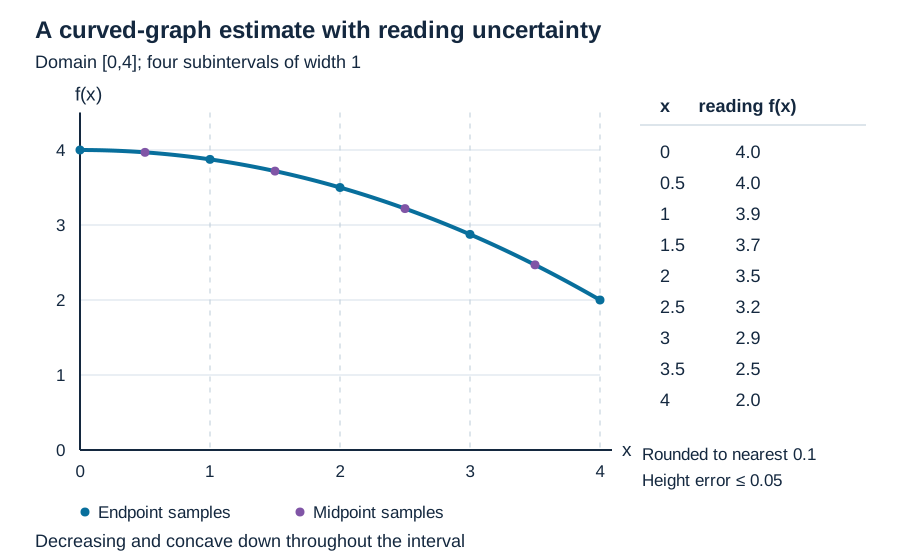
The supplied graph of f is continuous, strictly decreasing and strictly concave down throughout [0,4]. The accessible readings, rounded to the nearest 0.1, are: x = 0,0.5,1,1.5,2,2.5,3,3.5,4; f(x) ≈ 4.0,4.0,3.9,3.7,3.5,3.2,2.9,2.5,2.0 in that order. Each displayed height has at most 0.05 reading error. No formula for this curve is supplied.
Use the displayed readings for numerical estimates; each height has at most 0.05 reading error.Inspect diagram labels
The diagram keeps its full size here. Focus the view and use the arrow keys, or scroll across it, to inspect every label.
(a)Using the supplied curved graph readings, write the partition and width for four equal subintervals of [0,4]. Calculate left, right, midpoint and trapezoidal estimates of ∫₀⁴ f(x) dx, displaying the height-and-width expressions. Explain why these numbers are estimates rather than exact areas.
(b)Compute the two-subinterval trapezoidal estimate using x = 0,2,4 and compare it with T₄. State the left/right and trapezoid/midpoint error directions for exact heights, using the supplied monotonicity and concavity. Bound the effect of reading uncertainty on each four-subinterval estimate. Decide whether [13.3,13.4] is a guaranteed interval containing the integral, and whether |T₄ − T₂| is a rigorous error bound.
(c)As an analytic transfer, let r(t) = 1 + t² liters per minute for 0 ≤ t ≤ 2. Use two equal midpoint subintervals to approximate the accumulated volume ∫₀² r(t) dt. Use the behavior of r to determine whether that midpoint estimate is an underestimate or overestimate, and check using an exact integral.
Diagnose an estimate from a verbal rate description
Calculator optional
A continuous flow rate is positive and strictly concave up on the entire time interval [0,2] minutes. Its exact values at t = 0,1,2 are 1,2,4 liters per minute. Use one trapezoid on each of [0,1] and [1,2].
(a)Which choice gives the two-trapezoid estimate of the accumulated volume and a valid comparison with the true integral? Calculate the estimate and justify the direction from the stated whole-interval behavior.
Build an accumulation function from an integrand graph
Calculator optional
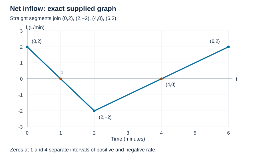
The exact graph of the continuous net inflow rate f is made of straight segments joining (0,2), (2,−2), (4,0) and (6,2), in that order. Time is measured in minutes and f in liters per minute. A tank contains 10 liters at t = 0. Define G to mean net change since time 0, and A to mean the amount in the tank.
The graph gives a signed net inflow rate, including negative rates.Inspect diagram labels
The diagram keeps its full size here. Focus the view and use the arrow keys, or scroll across it, to inspect every label.
(a)Before computing areas or inferring behavior, construct defining definite-integral expressions for G(x) and A(x) for 0 ≤ x ≤ 6. Identify the reference time, the variable endpoint and the role of the initial 10 liters.
(b)Use signed areas from the supplied integrand graph to compute G(0), G(1), G(2), G(4), G(6) and A(6). State the units. Then determine the absolute maximum and minimum of G on [0,6], comparing the endpoint values as well as interior candidates.
(c)Using the graph of f and the Fundamental Theorem of Calculus, determine where G increases and decreases, where G is concave up and concave down, and every inflection point of G. Explain separately how the sign of f and the increasing/decreasing behavior of f lead to those conclusions. Address the corner of f at x = 2.
(d)Sketch G on [0,6]. Label the five points found in part b, the horizontal tangents and the inflection point. Make your sketch agree with both the monotonicity and the concavity found in part c; explain why G can increase while its value is negative.
Accumulate a nonuniform rate table under a stated model
Calculator optional
A continuous rate is sampled at the exact pairs (t,f(t)) = (0,2), (1,4), (3,−2), (4,0), with time in minutes and rate in liters per minute. For parts a–c, explicitly assume linear interpolation between each pair of consecutive rows; call that rate model f_PL. The net change is measured from time 0.
(a)Construct the defining definite integral for G(x), the accumulated net change in the piecewise-linear model, for 0 ≤ x ≤ 4. State the reference and variable endpoint. Then compute G(1), G(3) and G(4) from the nonuniform table, showing the width of each interval and explaining why trapezoidal areas are exact for this model.
(b)Using only the supplied table and the stated linear-interpolation model, locate each zero of f_PL. Determine where G increases and decreases, find its absolute maximum and minimum on [0,4], and determine its concavity intervals and inflection points. Show the interpolated zero calculation and the signed area needed for the interior extreme value.
(c)Now remove the interpolation assumption and retain only continuity and the four table rows. Decide which conclusions still hold: G′(1) = 4, the exact value G(4) = 4, increase on the whole interval (0,7/3), and concavity changes at 1 and 3. Explain what sampled values do and do not determine, and identify the status of the sum 3 + 2 − 1.
Transfer accumulation reasoning to a formula and words
Calculator optional
For parts a–b, h(t) = t² − 2t on [0,3] and net accumulation is measured from t = 1. For parts c–d, r is continuous, strictly negative and strictly increasing on the entire interval [2,5]; its numerical values are not supplied.
(a)First construct H(x) as a definite integral of the supplied formula from the stated reference to x, for 0 ≤ x ≤ 3. Then obtain an explicit expression and compute H(0), H(1), H(2) and H(3). Explain why h(1) and H(1) need not be equal.
(b)From the analytic integrand h, determine where H increases and decreases, its concavity intervals, all inflection points, and its absolute maximum and minimum on [0,3]. Justify each conclusion through the integrand’s sign or trend and compare endpoints for absolute extrema.
(c)For the verbally described rate r, construct S(x), its net accumulation from time 2 to x, for 2 ≤ x ≤ 5. State S(2) and explain why no exact number for S(5) can be obtained from the description alone.
(d)Use the whole-interval verbal hypotheses to determine the sign of S(x) for x > 2, whether S increases or decreases, and its concavity. Explain how a negative but increasing integrand can produce the behavior you describe.
A continuous rate f has exact samples f(0) = 2, f(1) = 4 and f(2) = 6. No interpolation, monotonicity or concavity assumption is supplied. Let G(x) = ∫₀ˣ f(t) dt.
(a)Which conclusion is justified by these hypotheses? Explain your choice using the defining integral and FTC, and identify why the other claims would need additional information between sampled times.