Skip to the reading

Chapter 7 Solutions

Worked solutions to all thirty problems, with the reason for each step. These explanations were added for this edition; the chapter answer key and original worked examples follow below.

Chapter problems → · Chapter answer key →

Problem 1

Original problem · added worked solution

For questions 1-3, determine the value of the expansion

Original source equation or figure

The powers in the source expansion are $(3π/2)^{2n}$ with denominator $(2n)!$ and alternating signs.
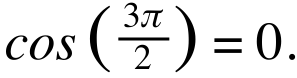
This is $cos(3π/2)$ by the cosine Maclaurin series, which converges for every real argument.
The unit-circle value is $cos(3π/2)=0$ .

Final answer

$0$ .

Return to problem 1 →

Problem 2

Original problem · added worked solution

For questions 1-3, determine the value of the expansion

Original source equation or figure

The expansion is $∑_{n=0}^{∞}420^n/n!$ .
This is the exponential Maclaurin series at x=420. Its radius is infinite, so the value is $e^{420}$ .

Final answer

$e^{420}$ .

Return to problem 2 →

Problem 3

Original problem · added worked solution

For questions 1-3, determine the value of the expansion

Original source equation or figure

The powers are $(2π)^{2n+1}$ , with alternating signs and factorial denominators $(2n+1)!$ .
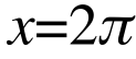
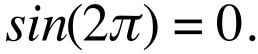
This is the sine Maclaurin series at x=2π, convergent for every real x.
Therefore the expansion equals $sin(2π)=0$ .

Final answer

$0$ .

Return to problem 3 →

Problem 4

Original problem · added worked solution

For questions 4 and 5, evaluate the infinite sum

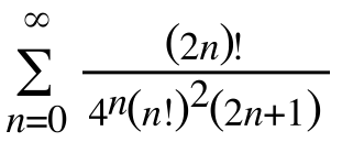
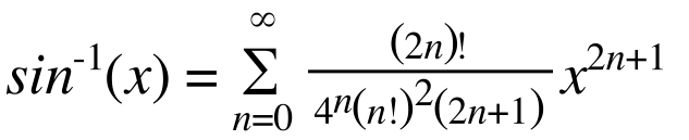
Original source equation or figure

The arcsine expansion is $arcsin x=∑_{n=0}^{∞}(2n)!x^{2n+1}/(4^n(n!)^2(2n+1))$ for $|x|<1$ .
The source sum is its endpoint x=1. The coefficients behave as a constant times $n^{-3/2}$ , so the endpoint series converges. Equivalently, integrate the positive binomial expansion of $1/sqrt(1-x^2)$ up to 1 using monotone convergence.
Its value is the endpoint integral $∫_0^1 dx/sqrt(1-x^2)=arcsin1=π/2$ .

Final answer

$π/2$ .

Return to problem 4 →

Problem 5

Original problem · added worked solution

For questions 4 and 5, evaluate the infinite sum

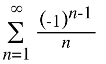
Original source equation or figure

The given series is $1-1/2+1/3-1/4+…$ .
It converges by the alternating series test. The logarithmic expansion $ln(1+x)=∑_{n=1}^{∞}(-1)^{n-1}x^n/n$ also converges at x=1.
Substitute x=1 to obtain $ln2$ , approximately 0.693147.

Final answer

$ln2≈0.693147$ .

Return to problem 5 →

Problem 6

Original problem · added worked solution

The average liger weighs 6.2lbs at birth. One standard deviation is approximately 1.2lbs.

What is the probability of a liger weighing between 5 and 6.2 lbs?

The question supplies mean and standard deviation; this solution uses the normal-distribution model introduced in the chapter. Original answer prose sometimes switches pounds to ounces; the prompt’s pounds are retained.

Use the normal model described in this chapter, with mean $μ=6.2$ pounds and standard deviation $σ=1.2$ pounds. Mean and standard deviation alone would not determine this probability without a distribution assumption.
Standardize with $z=(w-6.2)/1.2$ . The endpoints 5 and 6.2 become $a=-1$ and $b=0$ .
The probability is $(1/sqrt(2π))∫_{-1}^{0}e^{-z^2/2}dz$ . Expand $e^{-z^2/2}=∑_{n=0}^{∞}(-1)^n z^{2n}/(2^n n!)$ and integrate term by term on this finite interval.
This yields $(1/sqrt(2π))∑_{n=0}^{∞}(-1)^n(b^{2n+1}-a^{2n+1})/(2^n n!(2n+1))$ . Evaluation gives $0.341344746$ , or approximately 34.1345%.

Final answer

Under the normal model, $P≈0.341344746$ .

Return to problem 6 →

Problem 7

Original problem · added worked solution

The average liger weighs 6.2lbs at birth. One standard deviation is approximately 1.2lbs.

What is the probability of a liger weighing between 6.8 and 7.4 lbs?

Use the normal model described in this chapter, with mean $μ=6.2$ pounds and standard deviation $σ=1.2$ pounds. Mean and standard deviation alone would not determine this probability without a distribution assumption.
Standardize with $z=(w-6.2)/1.2$ . The endpoints 6.8 and 7.4 become $a=0.5$ and $b=1$ .
The probability is $(1/sqrt(2π))∫_{0.5}^{1}e^{-z^2/2}dz$ . Expand $e^{-z^2/2}=∑_{n=0}^{∞}(-1)^n z^{2n}/(2^n n!)$ and integrate term by term on this finite interval.
This yields $(1/sqrt(2π))∑_{n=0}^{∞}(-1)^n(b^{2n+1}-a^{2n+1})/(2^n n!(2n+1))$ . Evaluation gives $0.149882285$ , or approximately 14.9882%.

Final answer

Under the normal model, $P≈0.149882285$ .

Return to problem 7 →

Problem 8

Original problem · added worked solution

The average liger weighs 6.2lbs at birth. One standard deviation is approximately 1.2lbs.

What is the probability of a liger weighing between 3.8 and 8.6 lbs?

Use the normal model described in this chapter, with mean $μ=6.2$ pounds and standard deviation $σ=1.2$ pounds. Mean and standard deviation alone would not determine this probability without a distribution assumption.
Standardize with $z=(w-6.2)/1.2$ . The endpoints 3.8 and 8.6 become $a=-2$ and $b=2$ .
The probability is $(1/sqrt(2π))∫_{-2}^{2}e^{-z^2/2}dz$ . Expand $e^{-z^2/2}=∑_{n=0}^{∞}(-1)^n z^{2n}/(2^n n!)$ and integrate term by term on this finite interval.
This yields $(1/sqrt(2π))∑_{n=0}^{∞}(-1)^n(b^{2n+1}-a^{2n+1})/(2^n n!(2n+1))$ . Evaluation gives $0.954499736$ , or approximately 95.4500%.

Final answer

Under the normal model, $P≈0.954499736$ .

Return to problem 8 →

Problem 9

Original problem · added worked solution

For the next five questions, evaluate the definite integrals using a five-term Taylor Expansion

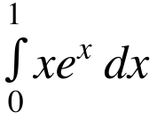
Original source equation or figure

Use the first five nonzero terms of $e^x≈1+x+x^2/2+x^3/6+x^4/24$ .
Multiply by x to approximate $xe^x$ by $x+x^2+x^3/2+x^4/6+x^5/24$ .
Integrating from 0 to 1 gives $1/2+1/3+1/8+1/30+1/144=719/720≈0.998611111$ .
This is a five-term approximation. The exact integral is 1, so its actual error is $1/720≈0.001388889$ .

Final answer

Five-term approximation $719/720≈0.998611111$ .

Return to problem 9 →

Problem 10

Original problem · added worked solution

For the next five questions, evaluate the definite integrals using a five-term Taylor Expansion

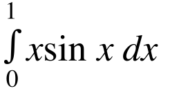
Original source equation or figure

Use $sin x≈x-x^3/6+x^5/120-x^7/5040+x^9/362880$ .
Multiply by x and integrate each monomial from 0 to 1: $1/3-1/30+1/840-1/45360+1/3991680$ .
The value is $400723/1330560≈0.301168681$ . This is an approximation; the exact integral is $sin1-cos1$ .
The next integrated magnitude is $1/(11!·13)$ , which bounds the error because the integrated terms alternate and decrease.

Final answer

Approximately $0.301168681$ .

Return to problem 10 →

Problem 11

Original problem · added worked solution

For the next five questions, evaluate the definite integrals using a five-term Taylor Expansion

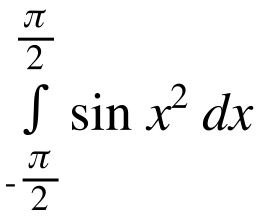
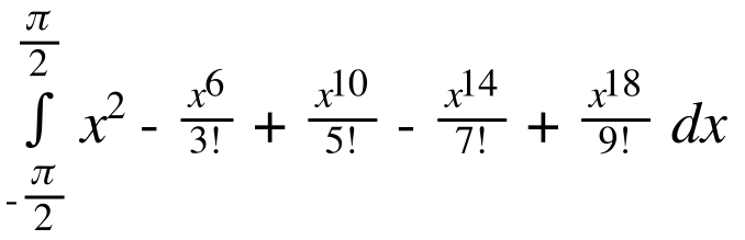
Original source equation or figure

Read the source integrand as $sin(x^2)$ . Substitute x² into the sine expansion to obtain $x^2-x^6/6+x^{10}/120-x^{14}/5040+x^{18}/362880$ .
These terms are even functions, so the integral over $-π/2≤x≤π/2$ is twice the integral from 0 to $π/2$ . Set $a=π/2$ .
Termwise integration gives $2(a^3/3-a^7/42+a^{11}/1320-a^{15}/75600+a^{19}/6894720)$ .
This five-term value is approximately $1.656300984$ . The sine expansion converges uniformly on this finite interval, justifying the full-series method; the five-term value remains an approximation.

Final answer

Approximately $1.656300984$ .

Return to problem 11 →

Problem 12

Original problem · clarified · added worked solution

For the next five questions, evaluate the definite integrals using a five-term Taylor Expansion

$∫_0^{1/2}xln(1+x)dx$

Corrected calculation: integrating the fifth term x⁶/5 gives x⁷/35. The five-term value rounds to 0.0355.

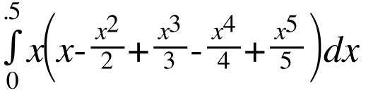
On $0≤x≤1/2$ , the first five nonzero Taylor terms are $ln(1+x)≈x-x^2/2+x^3/3-x^4/4+x^5/5$ .
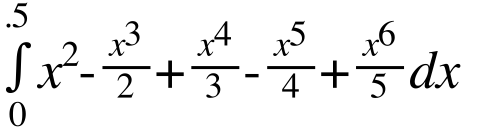
Multiplying by x gives $xln(1+x)≈x^2-x^3/2+x^4/3-x^5/4+x^6/5$ . Integrating term by term gives $x^3/3-x^4/8+x^5/15-x^6/24+x^7/35$ . In particular, $∫x^6/5 dx=x^7/35$ .
Evaluate this antiderivative between 0 and 1/2: $(1/2)^3/3-(1/2)^4/8+(1/2)^5/15-(1/2)^6/24+(1/2)^7/35=1909/53760≈0.035509672619$ .
Rounded to four decimal places, the five-term approximation is $0.0355$ . The first omitted integrated magnitude is $(1/2)^8/48≈0.000081381$ , which bounds the alternating truncation error.

Final answer

Five-term approximation $1909/53760≈0.035509672619$ , or $0.0355$ to four decimal places.

Return to problem 12 →

Problem 13

Original problem · added worked solution

For the next five questions, evaluate the definite integrals using a five-term Taylor Expansion

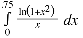
Original source equation or figure

For $0≤x≤0.75$ , substitute x² into $ln(1+u)$ . After dividing by x, the first five nonzero terms are $x-x^3/2+x^5/3-x^7/4+x^9/5$ . At zero the quotient has continuous limiting value zero.
Integrate to $a=0.75$ : $a^2/2-a^4/8+a^6/18-a^8/32+a^{10}/50$ .
This yields approximately $0.249584656$ . The next integrated magnitude $a^{12}/72≈0.000439949$ bounds the alternating truncation error.

Final answer

Approximately $0.249584656$ .

Return to problem 13 →

Problem 14

Added problem and worked solution

Evaluate $∑_{n=0}^{∞}1/n!$ .

The exponential expansion is $e^x=∑_{n=0}^{∞}x^n/n!$ .
Setting x=1 gives $∑1/n!=e$ . Convergence follows from its infinite radius.

Final answer

$e$ .

Return to problem 14 →

Problem 15

Added problem and worked solution

Evaluate $∑_{n=0}^{∞}(-1)^n/(2n)!$ .

The cosine expansion is $cos x=∑_{n=0}^{∞}(-1)^n x^{2n}/(2n)!$ .
Setting x=1 gives the source sum, so its value is $cos1$ .

Final answer

$cos1$ .

Return to problem 15 →

Problem 16

Added problem and worked solution

Evaluate $∑_{n=1}^{∞}(-1)^{n+1}/(n2^n)$ .

The logarithmic series $ln(1+x)=∑_{n=1}^{∞}(-1)^{n+1}x^n/n$ converges for $-1<x≤1$ .
Substitute $x=1/2$ , which is strictly inside the convergence interval. The sum is $ln(3/2)$ .

Final answer

$ln(3/2)$ .

Return to problem 16 →

Problem 17

Added problem and worked solution

Evaluate $∑_{n=1}^{∞}n/n!$ .

For $n≥1$ , $n/n!=1/(n-1)!$ .
Let $k=n-1$ . The sum becomes $∑_{k=0}^{∞}1/k!=e$ . The index change preserves all terms.

Final answer

$e$ .

Return to problem 17 →

Problem 18

Added problem and worked solution

Evaluate $∑_{n=0}^{∞}1/(n+1)!$ .

Let $k=n+1$ . Then the sum is $∑_{k=1}^{∞}1/k!$ .
The full exponential sum at 1 is e; its k=0 term is 1. Subtract that term.

Final answer

$e-1$ .

Return to problem 18 →

Problem 19

Added problem and worked solution

Evaluate $∑_{n=0}^{∞}(-1)^n π^{2n+1}/(6^{2n+1}(2n+1)!)$ .

Recognize the sine expansion at $x=π/6$ . Its odd powers are $(π/6)^{2n+1}$ .
The sine series has infinite radius. The sum is $sin(π/6)=1/2$ .

Final answer

$1/2$ .

Return to problem 19 →

Problem 20

Added problem and worked solution

Use four Maclaurin terms to approximate $∫_0^{1/2}e^x dx$ , and give an error bound.

Use four terms: $e^x≈1+x+x^2/2+x^3/6$ .
Integrating from 0 to 1/2 gives $1/2+1/8+1/48+1/384=83/128=0.6484375$ .
Taylor’s pointwise remainder is at most $e^{1/2}x^4/4!$ . Integrating gives an error at most $e^{1/2}(1/2)^5/120≈0.000429355$ .

Final answer

$0.6484375$ , with error at most approximately $0.000429355$ .

Return to problem 20 →

Problem 21

Added problem and worked solution

Use five Maclaurin terms to approximate $∫_0^1e^{-x^2}dx$ , and bound the error.

Substitute $u=-x^2$ into the exponential series. Five terms give $e^{-x^2}≈1-x^2+x^4/2-x^6/6+x^8/24$ .
Integrate from 0 to 1 to obtain $1-1/3+1/10-1/42+1/216≈0.747486772$ .
The integrated series alternates with decreasing magnitudes. Its next term magnitude is $1/(5!·11)=1/1320$ , which bounds the error.

Final answer

Approximately $0.747486772$ , with error at most $1/1320$ .

Return to problem 21 →

Problem 22

Added problem and worked solution

Use three nonzero Maclaurin terms to approximate $∫_0^{1/2}(sin x)/x dx$ , interpreting the value at zero by continuity.

For x≠0, divide $sin x=x-x^3/6+x^5/120-…$ by x. At x=0 the quotient has limiting value 1.
Integrate the first three terms $1-x^2/6+x^4/120$ from 0 to 1/2. This gives $1/2-(1/2)^3/18+(1/2)^5/600≈0.493107639$ .
The first omitted integrated magnitude is $(1/2)^7/(7!·7)$ , so the error is at most approximately $0.000000221443$ .

Final answer

Approximately $0.493107639$ .

Return to problem 22 →

Problem 23

Added problem and worked solution

Use four nonzero Maclaurin terms to approximate $∫_0^{1/2}ln(1+x)dx$ , and bound the error.

Use $ln(1+x)≈x-x^2/2+x^3/3-x^4/4$ .
Integration from 0 to 1/2 gives $(1/2)^2/2-(1/2)^3/6+(1/2)^4/12-(1/2)^5/20=0.1078125$ .
The next integrated magnitude is $(1/2)^6/30=1/1920$ , bounding the alternating error.

Final answer

$0.1078125$ , with error at most $1/1920$ .

Return to problem 23 →

Problem 24

Added problem and worked solution

Approximate $∫_0^1 cos x dx$ with three nonzero Maclaurin terms and bound the error.

The first three cosine terms are $1-x^2/2+x^4/24$ .
Integrating from 0 to 1 gives $1-1/6+1/120=101/120≈0.841666667$ .
The next integrated magnitude is $1/(6!·7)=1/5040$ , which bounds the alternating error.

Final answer

$101/120≈0.841666667$ , with error at most $1/5040$ .

Return to problem 24 →

Problem 25

Added problem and worked solution

Approximate $ln(1.2)$ with three nonzero Maclaurin terms and bound the error.

Use three terms of $ln(1+x)=x-x^2/2+x^3/3-…$ at $x=0.2$ .
The value is $0.2-0.02+0.008/3≈0.182666667$ .
The alternating terms decrease, so the next magnitude $0.2^4/4=0.0004$ bounds the error.

Final answer

Approximately $0.182666667$ , with error at most $0.0004$ .

Return to problem 25 →

Problem 26

Added problem and worked solution

A weight W is normally distributed with mean 10 kg and standard deviation 2 kg. Find $P(8≤W≤12)$ .

The interval is within one standard deviation of the mean, so standardization gives $-1≤Z≤1$ .
For a standard normal variable, the probability is $(1/sqrt(2π))∫_{-1}^1e^{-z^2/2}dz$ .
By symmetry this is twice the probability from 0 to 1, giving approximately $0.682689492$ . The same value follows by integrating the exponential series term by term.

Final answer

Approximately $0.682689492$ , or 68.2689%.

Return to problem 26 →

Problem 27

Added problem and worked solution

A weight W is normally distributed with mean 10 kg and standard deviation 2 kg. Find $P(W≥12)$ .

Standardize 12 kg: $z=(12-10)/2=1$ .
Symmetry gives $P(Z≥1)=1/2-P(0≤Z≤1)$ .
Using the normal integral or its Taylor-series evaluation, $P(0≤Z≤1)≈0.341344746$ , so the upper tail is approximately $0.158655254$ .

Final answer

Approximately $0.158655254$ .

Return to problem 27 →

Problem 28

Added problem and worked solution

A normally distributed random variable has mean μ. What is $P(X≤μ)$ ? Explain.

A normal density is symmetric around its mean.
Half the total probability lies below the mean and half above it. A single point has probability zero.

Final answer

$1/2$ .

Return to problem 28 →

Problem 29

Added problem and worked solution

Let X be normally distributed with mean 100 and standard deviation 15. Use a standardized integral or series to find $P(100≤X≤115)$ .

Set $Z=(X-100)/15$ . The endpoints 100 and 115 become 0 and 1.
Thus the probability is $(1/sqrt(2π))∫_0^1e^{-z^2/2}dz$ .
Expanding the exponential and integrating produces $(1/sqrt(2π))∑_{n=0}^{∞}(-1)^n/(2^n n!(2n+1))≈0.341344746$ .

Final answer

Approximately $0.341344746$ .

Return to problem 29 →

Problem 30

Added problem and worked solution

Do a mean and a standard deviation alone determine an interval probability? Explain with an example.

Mean and standard deviation describe only two features of a distribution. They do not specify its full shape.
For example, a normal variable with mean 0 and standard deviation 1 has $P(-1/2≤X≤1/2)≈0.382925$ . A variable taking −1 and 1 with equal probability has the same mean and standard deviation but probability zero in that interval.
Therefore a normal model or other distribution information is needed for the specific integral-based answer.

Final answer

No; distributions with the same mean and standard deviation can assign different probabilities to an interval.

Return to problem 30 →

Chapter answer key and worked steps

Answers and worked steps for the original problems, including verified corrections where needed.

Original worked answer

=
The expansion follows the series..
,
where x= . Therefore,

Problem 1 →
Original worked answer

The expansion follows the series...
ex ≈
where x=420. Therefore, the expansion is equal to
e420
Problem 2 →
Original worked answer

=

The expansion follows the series...
,
where . Therefore,

Problem 3 →
Original worked answer

The summation follows the series..

Where x=1. Therefore,
sin-1(1) = .
Problem 4 →
Original worked answer

The summation follows the alternating harmonic series. Expanding the summation...

The expansion follows the series...

where x=1. Therefore,
ln(2)=.693
Problem 5 →
Corrected units

A weight between 5 and 6.2 pounds falls one standard deviation from the norm.
The values for a and b are
a= -1, b=0. Plugging it into the formula..

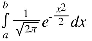
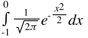. Using the exponential taylor series..

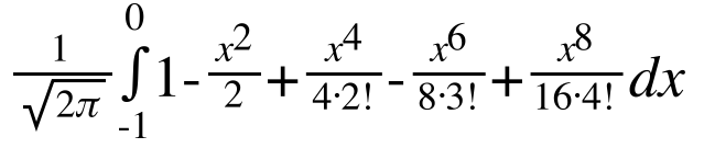
=34.1%
Problem 6 →
Corrected units

A weight between 6.8 and 7.4 pounds falls between half and one standard deviation from the norm.
The values for a and b are
a= .5, b=1. Plugging it into the formula..

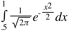. Using the exponential taylor series..

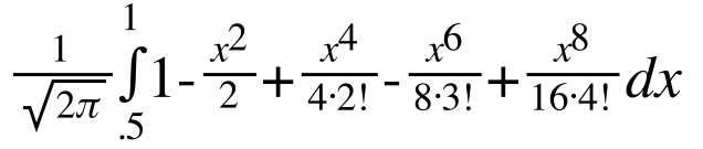
=14.99%
Problem 7 →
Corrected units

A weight between 3.8 and 8.6 pounds falls between two standard deviations to the left and right of the norm.
The values for a and b are
a= -2, b=2. Plugging it into the formula..

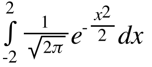. Using the exponential taylor series..

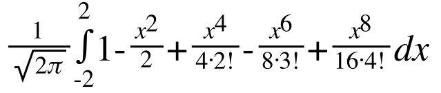
$(1/√(2π))[z−z^3/6+z^5/40−z^7/336+z^9/3456]_{−2}^{2}=2332/(945√(2π))$
The first five terms give 0.984479786, or about 98.44798%. This truncation is too coarse for the full probability. Using sixteen terms (n = 0 through 15) gives 0.954499736, or about 95.45%, with next-term error at most 1.515 × 10⁻¹⁰.

Problem 8 →
Original worked answer

Using a five-term expansion..

=
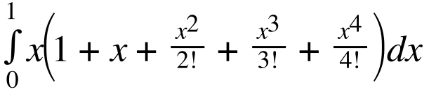
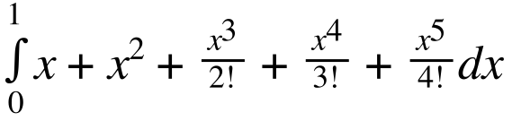
= .998
Problem 9 →
Corrected worked answer

Using a five-term expansion..

$x^2−x^4/3!+x^6/5!−x^8/7!+x^10/9!$
$x^3/3−x^5/(5⋅3!)+x^7/(7⋅5!)−x^9/(9⋅7!)+x^11/(11⋅9!)$
= $1/3−1/(5⋅3!)+1/(7⋅5!)−1/(9⋅7!)+1/(11⋅9!)$
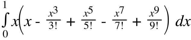
= .301168
Problem 10 →
Original worked answer

Using a five-term expansion..

`= 1.656
Problem 11 →
Corrected worked answer

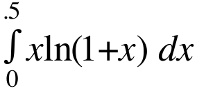
Using a five-term expansion..

$x^3/3-x^4/8+x^5/15-x^6/24+x^7/35$
= $(1/2)^3/3-(1/2)^4/8+(1/2)^5/15-(1/2)^6/24+(1/2)^7/35$
= .0355
Problem 12 →
Original worked answer

Using a five-term expansion..

=
=
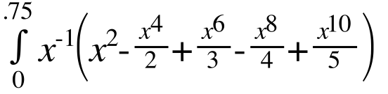
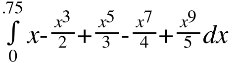
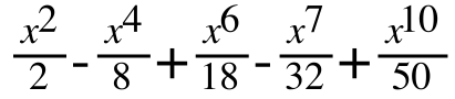
= .2496
Problem 13 →