Finding Taylor Polynomial Approximations of Functions
Build a center-specific Taylor polynomial from derivative values and label its value as an approximation.
College Board Topic 10.11 · CED p. 191 (PDF p. 196) · CED effective Fall 2020; project course outline 2026–27.
A Taylor polynomial matches a function’s value and its derivatives at a center a. Its degree-n form is . The constant term is f(a); the first term is the tangent-line approximation; higher terms add local curvature and further derivative information. A Maclaurin polynomial is centered at a=0.
The factorial belongs in every coefficient. A derivative value is not usually the coefficient itself: a second derivative of 4 gives coefficient 4/2!=2. The shift (x−a) belongs in every power. Near the center, a suitable higher-degree polynomial often improves the approximation; this is not a universal promise of better accuracy at every faraway point.
A derivative table can supply all the needed data without a formula for f. For , values , , , give . Evaluating at 2.1 gives 2.921. That is an approximation to f(2.1), not an exact function value unless f equals this polynomial.
Connect to the retained Taylor lesson and Maclaurin lesson. A graph of the function and its local polynomial helps explain the center; a bound in the next topic is what quantifies the error.
Let's work through it
- For sin x at a=0, derivative values through degree 3 are . Why: Differentiate sin repeatedly and evaluate at the center.
- . Why: Divide the third derivative by 3!, and include the zero even coefficients.
- . Why: Substitute a small x to get the polynomial approximation, not an equality to sin(0.2).
A whole interval needs a remainder that vanishes
A Taylor polynomial about a real center a is T_n(x) = Σ_(k=0)^n f⁽ᵏ⁾(a)(x−a)^k/k!. Finite derivative matching is local information. To establish that increasing-degree polynomials approach f over an interval I, control the remainder R_n(x) = f(x)−T_n(x) for every x in that interval.
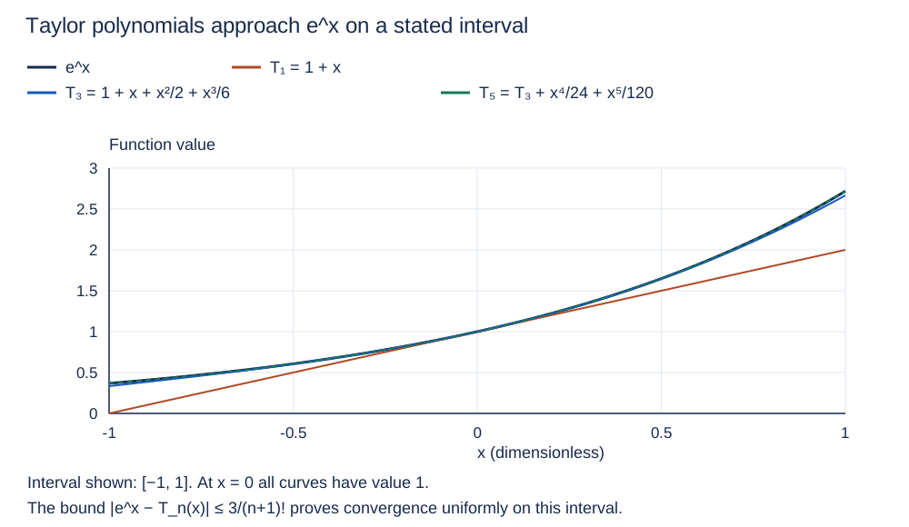
For f(x) = e^x centered at 0, every derivative at 0 is 1, so T_n(x) = Σ_(k=0)^n x^k/k!. Use the established remainder estimate |R_n(x)| ≤ M|x|^(n+1)/(n+1)! when the magnitude of the (n+1)st derivative is at most M between 0 and x. On I = [−1,1], all those derivative magnitudes are at most e < 3. Thus |e^x−T_n(x)| ≤ 3/(n+1)! for every x in [−1,1].
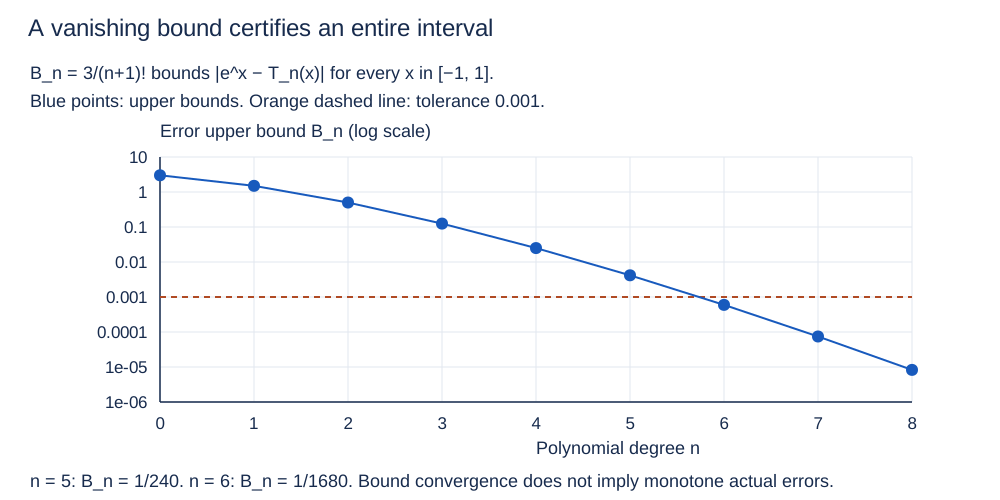
The bound tends to zero: successive bounds have ratio 1/(n+2), so factorial growth forces B_n = 3/(n+1)! → 0. Given any positive tolerance ε, choose one sufficiently large N so B_n < ε for every n ≥ N. The same N works for every x in the stated interval. This proves increasing-degree convergence over that interval, rather than just an improvement at one sampled point. The interval and derivative bound are part of the argument; the same number 3 must not be used on an unstated larger interval.
The graph illustrates T₁, T₃ and T₅. The formulas and vanishing bound establish the limit. A finite graph, finite derivative table, or a few favorable error comparisons alone cannot prove increasing-degree convergence.
Inspect diagram labels
The diagram keeps its full size here. Focus the view and use the arrow keys, or scroll across it, to inspect every label.
Inspect diagram labels
The diagram keeps its full size here. Focus the view and use the arrow keys, or scroll across it, to inspect every label.
A shrinking bound is not a promise about each actual error
An upper bound B_n describes a guaranteed ceiling for |f(x)−T_n(x)|. If B_n → 0 uniformly on an interval, the actual errors tend to zero there. This does not imply that every successive degree makes each actual error smaller. Upper bounds need not be sharp, and the added term may temporarily undo earlier cancellation.
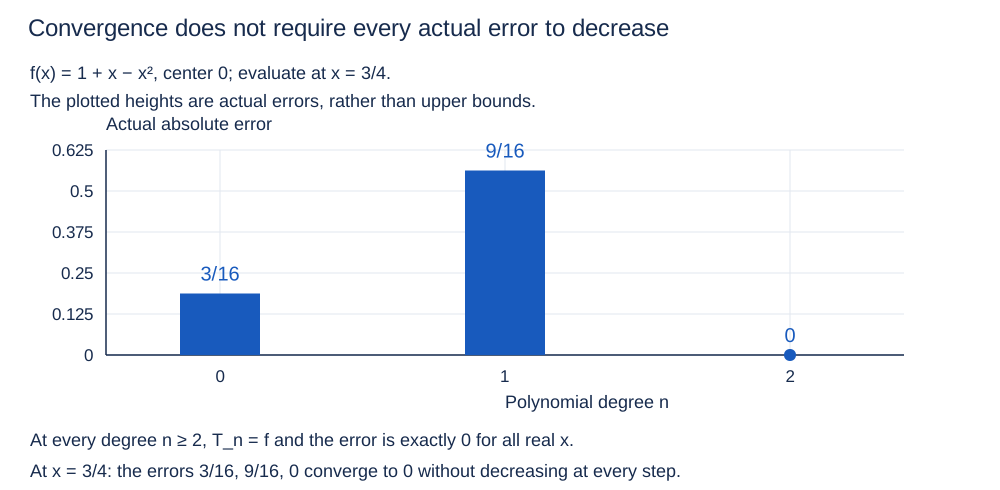
For f(x)=1+x−x² centered at 0, T₀=1, T₁=1+x, and T_n=f for every n ≥ 2. At x=3/4, f(x)=19/16. The actual errors are 3/16, 9/16, then 0. The error increases before vanishing. Nevertheless, T_n approaches f on [−1,1], and indeed on all real x, because its remainder is identically zero for every n ≥ 2.
The official approximation statement says “in many cases” and “over some interval.” Do not replace that with a universal theorem about every smooth function, every x, or monotone actual errors. Matching all derivatives at a center needs an appropriate vanishing-remainder argument before it establishes equality to the function away from the center.
Inspect diagram labels
The diagram keeps its full size here. Focus the view and use the arrow keys, or scroll across it, to inspect every label.
One degree can meet a tolerance at every point in an interval
For e^x centered at 0 on [−1,1], use e < 3 and the established Taylor remainder estimate to certify an absolute error of at most 0.001.
Inspect diagram labels
The diagram keeps its full size here. Focus the view and use the arrow keys, or scroll across it, to inspect every label.
Inspect diagram labels
The diagram keeps its full size here. Focus the view and use the arrow keys, or scroll across it, to inspect every label.
- The derivative values at 0 are all 1. Therefore T₁=1+x, T₃=1+x+x²/2+x³/6 and T₅=T₃+x⁴/24+x⁵/120.
- Every derivative is e^t, and for t between 0 and any x in [−1,1], e^t ≤ e < 3. Since |x| ≤ 1, |e^x−T_n(x)| ≤ 3/(n+1)! throughout the interval.
- B₅=3/6!=1/240≈0.0041667 exceeds 0.001; B₆=3/7!=1/1680≈0.000595238 is below it. Because B_n decreases with n, degree 6 is the smallest degree certified by this particular bound.
- B_(n+1)/B_n=1/(n+2) ≤ 1/2 for n≥0. Hence B_n ≤ 3(1/2)^n → 0, and the polynomials converge to e^x on [−1,1] with a bound valid at all points simultaneously.
- At x=1, T₃=8/3≈2.666667 and T₅=163/60≈2.716667; e≈2.718282. At x=−1, T₃=1/3 and T₅=11/30≈0.366667; e^(−1)≈0.367879. These checks illustrate the graph but are not the interval proof.
Answer and check
Degree 6 certifies error at most 0.001 throughout [−1,1]. All increasing degrees converge there because the common remainder bound tends to zero.
Convergence survives a temporary error increase
Analyze the Maclaurin sequence for f(x)=1+x−x² on [−1,1] and compare its actual errors at x=3/4.
Inspect diagram labels
The diagram keeps its full size here. Focus the view and use the arrow keys, or scroll across it, to inspect every label.
- At 0, the derivative values are 1, 1, −2, followed by zeros. Taylor coefficients are those values divided by k!, so T₀=1, T₁=1+x and T₂=1+x−x².
- For every n≥2, all additional Taylor coefficients are zero. T_n equals f exactly, so R_n(x)=0 throughout [−1,1] for all n≥2. This is a vanishing interval-wide error bound.
- At x=3/4, f=1+3/4−9/16=19/16. T₀=16/16 and T₁=28/16. Thus the actual errors are |19−16|/16=3/16 and |19−28|/16=9/16, followed by 0.
- The degree-1 actual error is three times the degree-0 error at this point, although the Taylor sequence subsequently becomes exact. Convergence does not require monotone actual-error reduction.
Answer and check
T_n=f for n≥2. At x=3/4, errors are 3/16, 9/16, 0, 0, … .
Try it from memory
Pause & retrieve
Try it before you peek.
Write your answer and the reason from memory. Then compare with the worked answer. Your self-assessment is a study decision, not an automatically graded score.
Question 1
See every recall question with its answer
These references preserve each prompt and its answer for direct evidence links. Try the interactive questions above before opening the worked reasoning.
Retrieval 1
Worked answer and reason
Divide by 2!.
Retrieval 2
Worked answer and reason
Maclaurin is the special Taylor center a=0.
Catch the tempting mistake
- Higher degree guarantees better approximation everywhere.
- Taylor approximations are local; accuracy depends on the point and a remainder bound, not degree alone.
Calculator workspace and limits
For calculus, set the angle selector to Radians. This scientific calculator evaluates arithmetic and functions. It does not graph arbitrary functions, find numerical roots, evaluate numerical derivatives, or compute definite integrals. Those tasks need an approved graphing tool; the May 2027 exam permits approved handheld graphing calculators and Bluebook’s built-in Desmos on calculator-required parts. A graph or decimal estimate helps you check a conclusion; your setup, hypotheses, units and justification still do the explaining.
Scientific calculator
This calculator requires JavaScript. Use the physics formula sheets and show your working manually.
+ − * / ^ ! · pi · e · sqrt · sin, cos, tan · asin, acos, atan · atan2(y,x) · ln, log · abs · exp · hypot(x,y). Use * between factors. Keep units in your written working.
Put it to work
- Unit 10 problem 21 · No calculator · numerical
- Unit 10 problem 22 · No calculator · multiple
- Unit 10 problem 23 · No calculator · analytic
Explain and apply the mathematics
Try these problems before opening the solutions. Show your setup, the hypotheses behind your method, and what your answer means.
Prove increasing-degree convergence on an entire interval
Let f(x)=e^x and T_n be its degree-n Maclaurin polynomial. Work on I=[−1,1]. You may use e<3 and the established remainder estimate |f(x)−T_n(x)|≤M|x|^(n+1)/(n+1)! whenever |f⁽ⁿ⁺¹⁾(t)|≤M for t between 0 and x. For sketching, e^(−1)≈0.367879, e^0=1 and e≈2.718282 are supplied.
(a) For e^x centered at 0, derive the coefficient of x^k from the kth derivative at 0. Write T₁, T₃ and T₅, then evaluate each at x=−1,0,1. Give exact polynomial values.
(b) Using the supplied remainder estimate, prove that T_n approaches e^x for every x in the entire interval [−1,1] as n increases. Establish a bound independent of x, show that it tends to zero, and explain why one sufficiently large degree works for any prescribed positive tolerance at every point in the interval.
(c) Sketch e^x and T₁,T₃,T₅ on the common interval [−1,1], with labeled axes and a legend. Use their three supplied or calculated values at −1,0,1 and the exact formulas to show the curve shapes. Explain what the plot illustrates and why it cannot replace the interval proof in part b.
(d) Find the smallest degree certified by B_n=3/(n+1)! to give absolute error at most 0.001 throughout [−1,1]. Compare the immediately preceding degree, and state whether this certificate proves that the actual error decreases at each degree for each x.
Written working workspace
Drawing is temporarily unavailable. Work on paper if needed, then record your reasoning here.
Saving written working requires JavaScript. Keep your work on paper or in your own notes; the source problem above remains available.
Worked solution and rubric →Revisit the explanation →Revisit the explanation →Revisit the explanation →
Construct a counterexample to monotone actual errors
Let f(x)=1+x−x², centered at 0, and let T_n be its Maclaurin polynomials. Compare actual errors on I=[−1,1], with a detailed check at x=3/4.
(a) Compute the derivative values at 0 and construct T₀,T₁,T₂. Evaluate f and those polynomials at x=3/4, then compute each actual absolute error. Does increasing degree from 0 to 1 improve the approximation at this point?
(b) For f(x)=1+x−x², determine T_n for every n≥2. Prove increasing-degree convergence to f throughout [−1,1] using an interval-wide remainder bound. Explain why the pointwise error increase in part a does not contradict this conclusion.
(c) Draw the actual absolute error versus degree at x=3/4 for degrees 0,1,2, using a labeled linear vertical scale. Mark what happens for all degrees n≥2. Interpret the graph as evidence against the claim that each larger degree must improve every pointwise approximation.
Written working workspace
Drawing is temporarily unavailable. Work on paper if needed, then record your reasoning here.
Saving written working requires JavaScript. Keep your work on paper or in your own notes; the source problem above remains available.
Worked solution and rubric →Revisit the explanation →Revisit the explanation →
What does a decreasing bound actually establish?
A proof establishes |e^x−T_n(x)|≤3/(n+1)! for every x in [−1,1]. The bound tends to zero as n increases.
(a) Given the bound |e^x−T_n(x)|≤3/(n+1)! throughout [−1,1], which conclusion necessarily follows as the degree increases?
Worked solution and rubric →Revisit the explanation →Revisit the explanation →
For the teacher
- Use derivative tables and center-shifted examples, not only memorized polynomials at zero. Assess approximation notation explicitly.
Glossary and deeper reading · 8 refreshers
These editorial refreshers supplement the reading. Definitions and examples are added guidance; original source wording and recorded answers remain in their original context.
-
Function
A mathematical function assigns exactly one output to each input in its domain. Inputs can share an output, but one input cannot have two different outputs. For example, f(x)=x² assigns the output 9 to both 3 and −3. Function notation names the rule and its input; f(3) means the output when the input is 3.
-
Derivative
A derivative gives the instantaneous rate of change of a function with respect to its input. At a point, it is the finite limit of the difference quotient when that limit exists. For example, the derivative of x² is 2x, so the tangent slope at x=3 is 6. A derivative function collects those rates across the inputs where the function is differentiable.
-
Factorial
The factorial n! multiplies the positive integers from 1 through n for a positive integer n. By definition, 0!=1. For example, 4!=4·3·2·1=24. Factorials occur in Taylor coefficients and their rapid growth often makes the ratio test useful.
-
Second derivative
A second derivative is the derivative of the first derivative. It measures how the first rate of change changes with the input; further repeated differentiation gives higher-order derivatives. For example, f(x)=x³ has f′(x)=3x² and f″(x)=6x. For position measured against time, the second derivative is acceleration.
-
Polynomial
A polynomial in one variable is a finite sum of constant multiples of nonnegative integer powers of that variable. The degree is the highest exponent with a nonzero coefficient. For example, 2x³−x+5 is a polynomial of degree 3. Expressions containing 1/x or √x are not polynomials in x.
-
Interval
An interval is a set of real numbers containing every number between any two of its members. Parentheses exclude an endpoint, while square brackets include it. For example, (1,4] includes 4 and every number between 1 and 4, but excludes 1. An infinite endpoint always uses a parenthesis because infinity is not a real endpoint.
-
Limit
A limit describes the value approached by outputs as inputs approach a specified target or grow without bound. For an input approaching a finite target, its value at that exact input does not determine the limit. For example, (x²−1)/(x−1) approaches 2 as x approaches 1 even though the original expression is undefined at 1. A finite two-sided limit requires the left and right approaches to agree.
-
Error bound
An error bound gives a justified upper limit for the magnitude of an approximation’s error. It states how far the approximate value can be from the true value. For example, an error bound of 0.01 places the true value within 0.01 of the approximation. A bound requires its stated hypotheses and is not a claim that the error actually equals the bound.