For Future Reference - Forces as Vectors
Original textbook reading.
Friction is a contact force that opposes relative sliding, or the tendency to slide, between two surfaces. We distinguish static friction before slip from kinetic friction during sliding.
Static friction magnitude obeys 0 ≤ fₛ ≤ μₛN (Equation 1.4.1), with fₛ,max = μₛN at impending slip. Kinetic friction in the simple sliding model has magnitude fₖ = μₖN. The coefficients depend on the contacting materials and conditions.
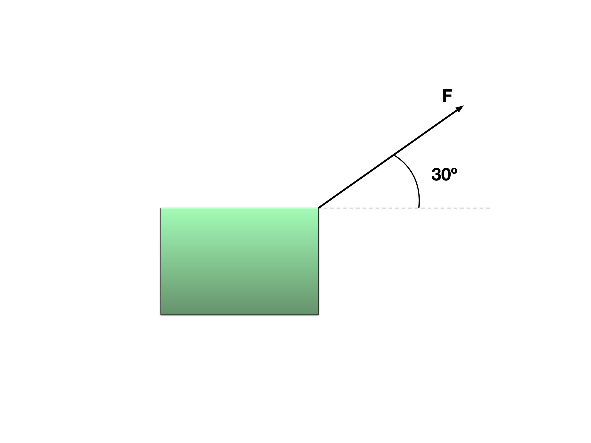
Notice how the Force here has a direction 30º North of East on the box. The length of the arrow signifies the magnitude of the Force, so the longer the arrow, the greater the magnitude
Read every step and figure
Step 1
Notice how the Force here has a direction 30º North of East on the box. The length of the arrow signifies the magnitude of the Force, so the longer the arrow, the greater the magnitude
Step 2
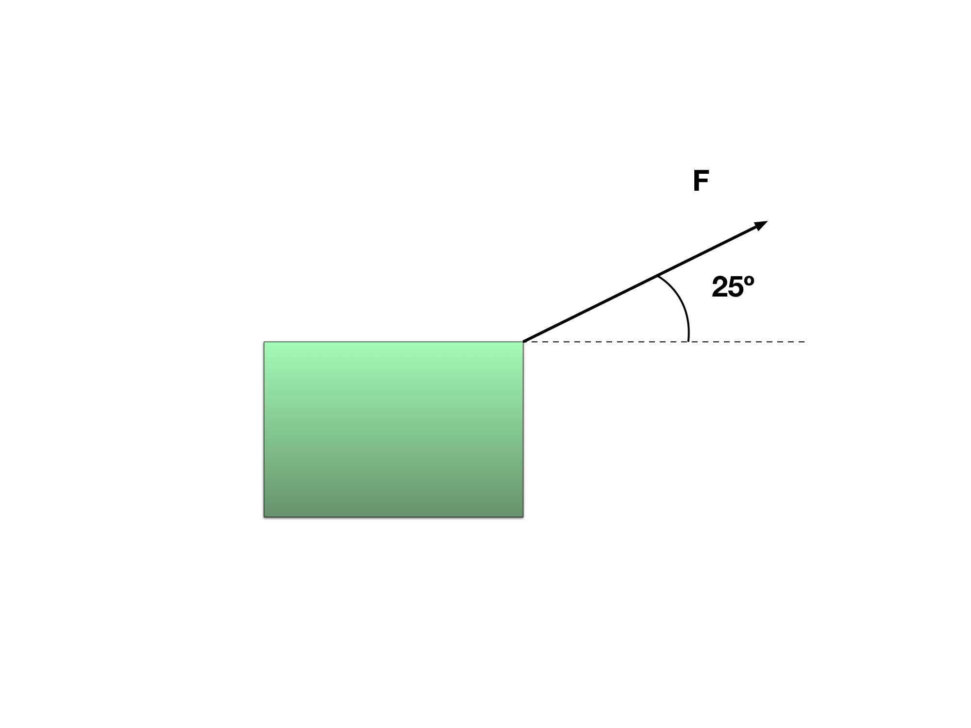
Notice in this one however that the magnitude of the force has changed, which is shown by the shorter arrow and the direction has changed as well to now 25º North of East.
Step 3
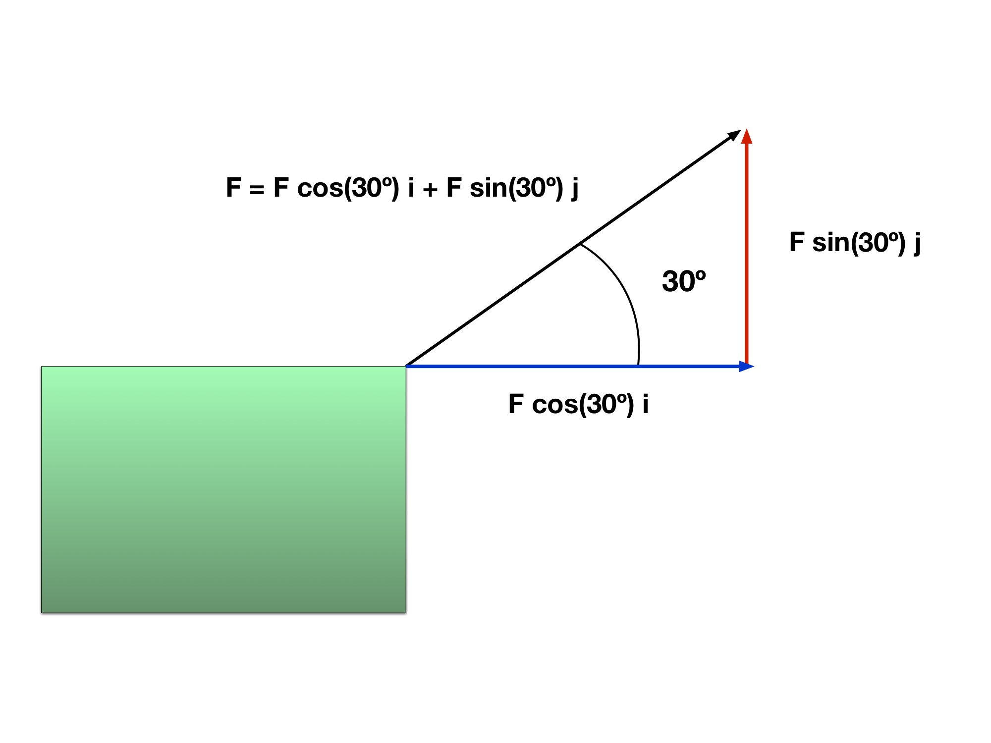
This picture represents the components of a force. It is the same as we discussed in sections 1 and 2. There is an i component (represented by the blue arrow) which is a vector along the x-axis and a j component (represented by the red arrow) which is the vector along the y-axis.
After adding the two vectors together, we get the resultant vector which is represented by the black arrow.
What if we expressed all of these forces as vectors? As we mentioned before, a vector is something that has direction and magnitudeⓘ. A force has both of these things! A force has a direction, i.e an object can be “pulled” or “pushed” a certain way. The magnitude of the force is associated with its relative “strength.” There are some forces that are stronger than others. Therefore they have a greater magnitude. Refer to Gallery 1.4.1 for an explanation on forces as vectors.
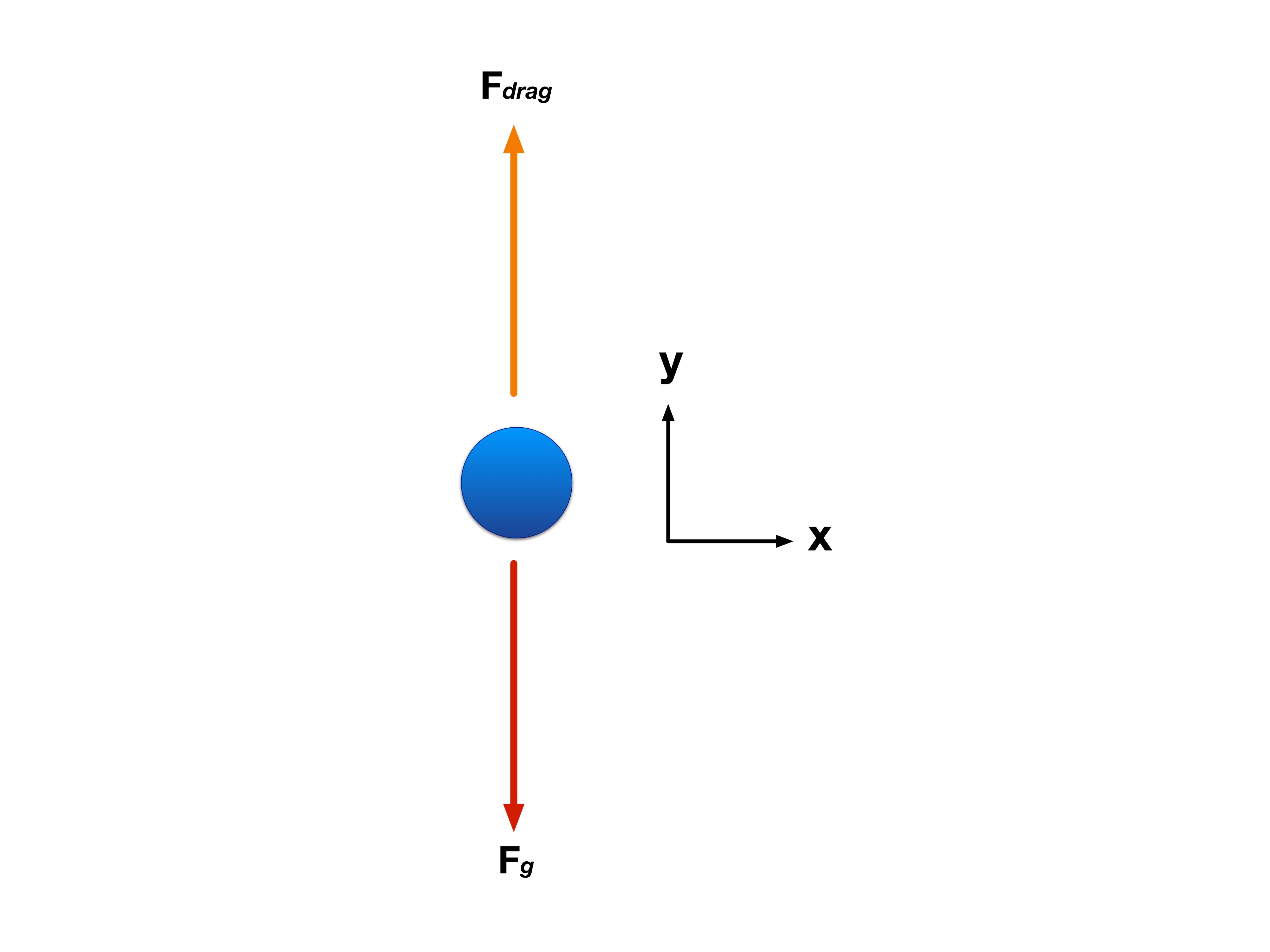
Something else to consider if we don’t want to represent the force as a vector is to break the force up into x and y components. For example, in Figure 1.4.1, there is a ball falling through the air where there is air resistance. There is a coordinate system in place for a point of reference/direction. The Figure is already constructed as an FBD.
Like we discussed in section 3, the ball is subject to a gravitational force denoted by , but what is new to this problem is the addition of a new force called drag force, which is a resistive force felt by an object when falling through an air medium. Remember Equation 1.3.1, and notice that in this example, we are dealing with multiple forces that act on an object. Therefore, a more proper way to approach this is thinking of things as a sum of forces that affect the object’s motion. So, a more proper way to write the force equation would be:
Figure 1.4.1 Falling Ball
(Equation 1.4.2)
Keep in mind that direction plays a role in this equation which is why we set a reference x and y-axes. The two forces acting on this ball are the drag force and the force of gravity. With this in mind, lets break this up into x and y components.
We’ve already mentioned that there are two forces acting in the y-direction. Based on this, we can say that the gravitational force is acting downwards in the negative y-direction while the Drag force is acting in the positive y-direction.
This is just Equation 1.4.2 applied to the y-direction. Keeping vector addition in mind:
Using scalar magnitudes with upward positive: F_drag − mg = maᵧ.
Notice here again that the force of gravity, is negative because its direction with respect to the reference y-axis is negative. Now let’s move on to the x-component. The equation we would use is:
(Equation 1.4.4)
In this equation, we do the same thing as we did for the y-component and analyze the forces acting on the object in the x-direction. However, do we have any forces in the x-direction? Based on our FBD in Figure 1.4.1, no! There are no forces acting in the x-direction, so there is no acceleration in the x-direction. Thus, the equation becomes:
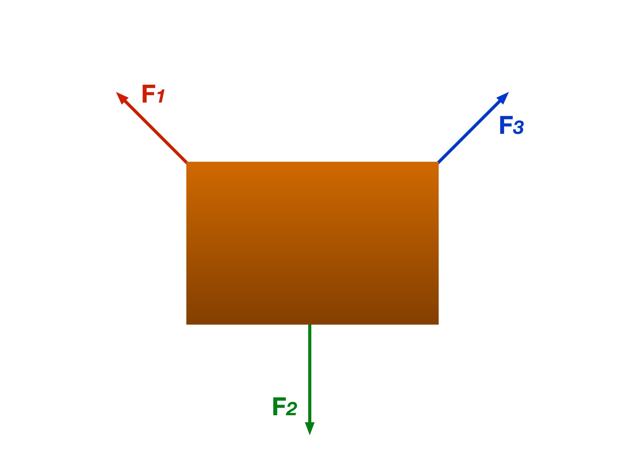
Let’s take a look at this box, with three different forces acting on it.
Read every step and figure
Step 1
Step 2
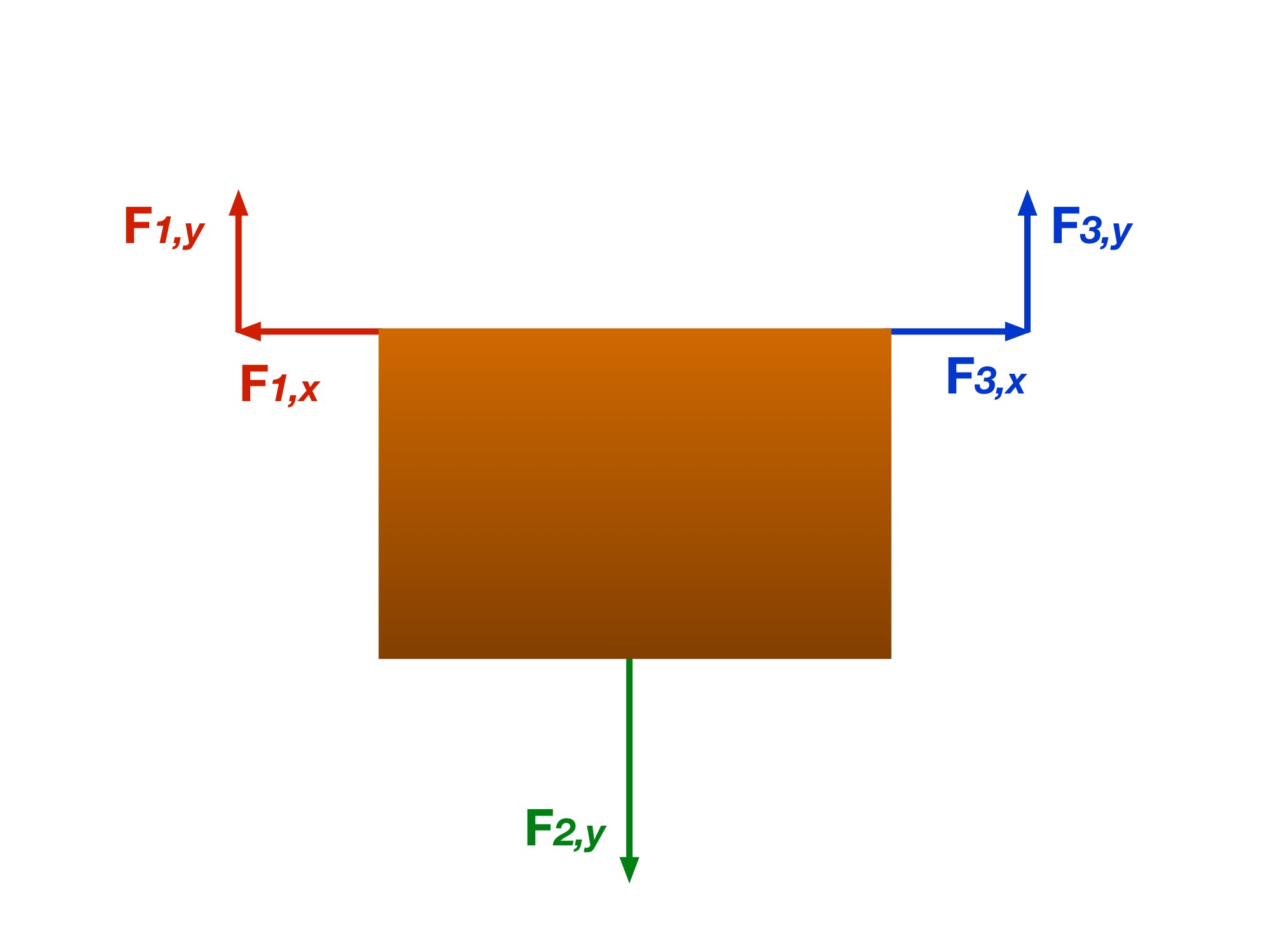
Step 3
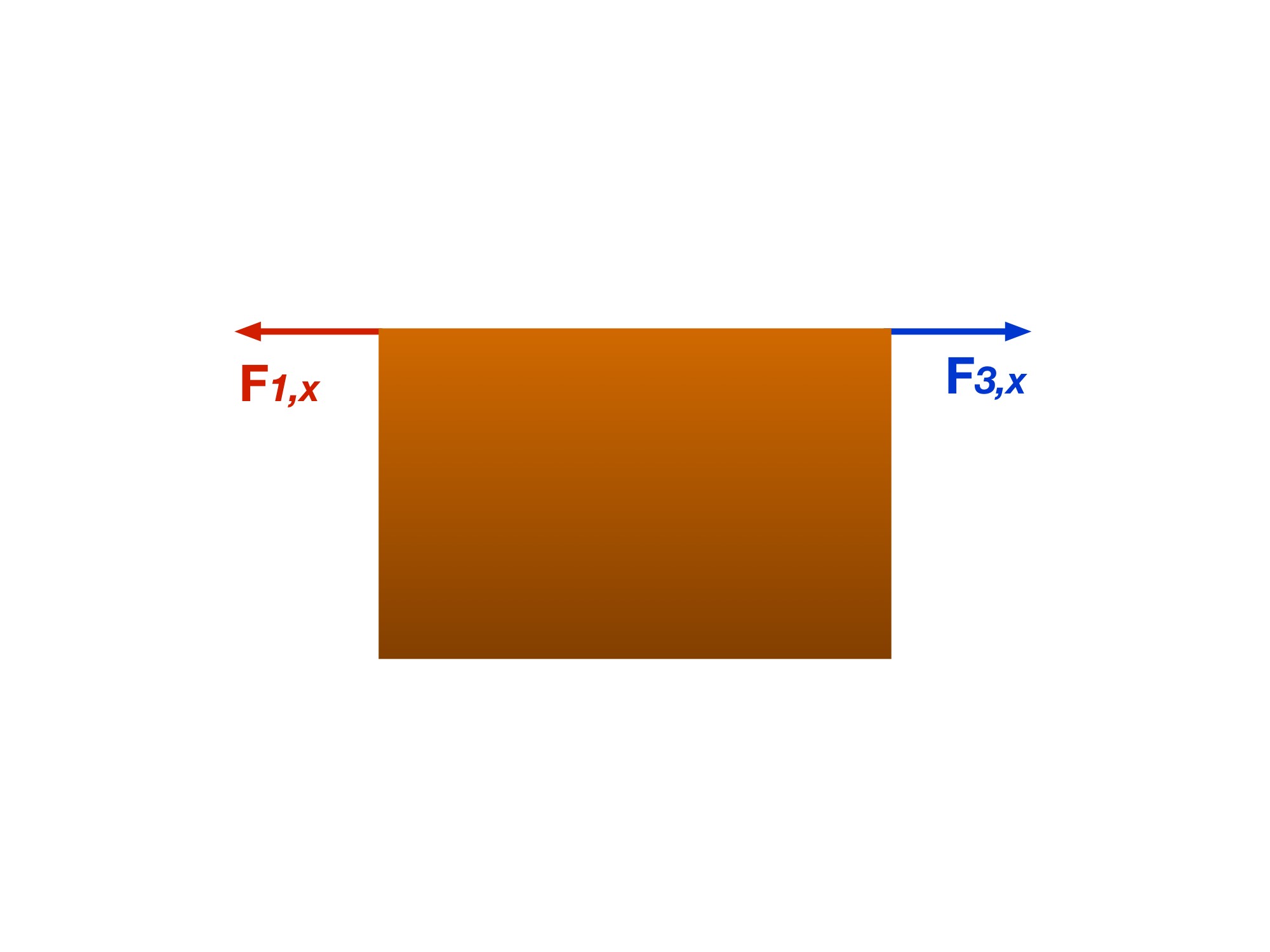
Step 4
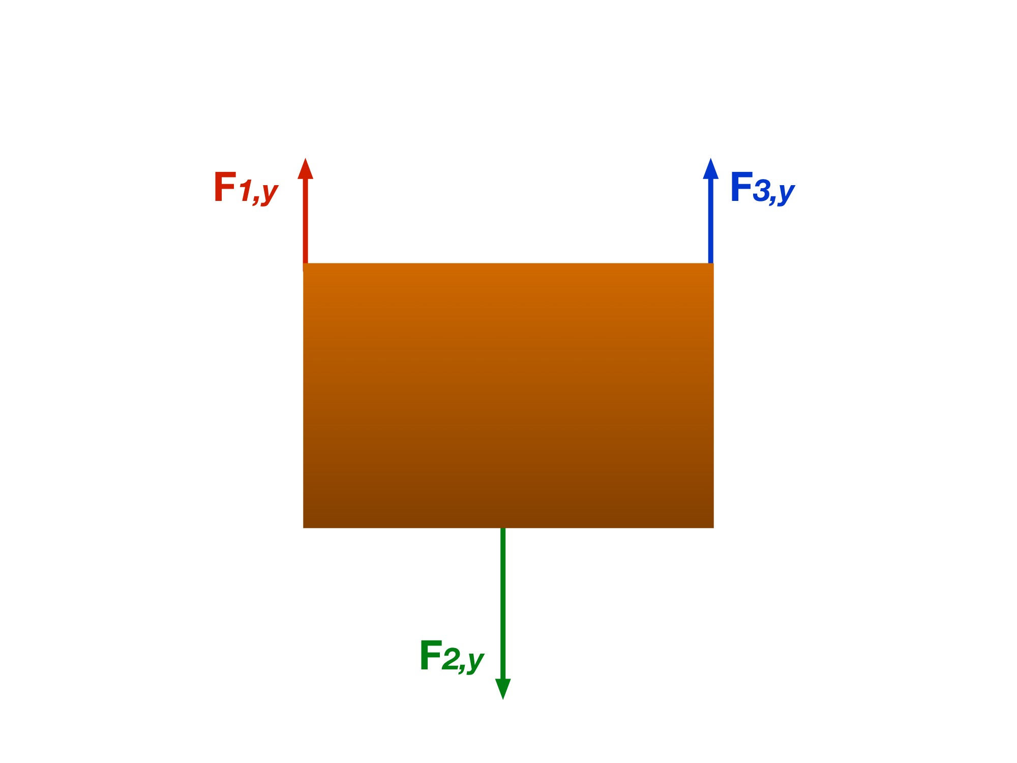
A man pulls a 3 kg cart with a force of 10 N at 25° above the horizontal. Model the cart as sliding to the right on a horizontal surface with kinetic-friction coefficient μₖ = 0.3 and zero vertical acceleration. Using g = 9.81 m/s², find its acceleration.
Step 1: Set up your Free Body Diagram
This is a crucial step in order to understand what’s going on in the given system. We know that the cart is moving towards the right, but in order to determine the acceleration, we must take into account all the forces acting on the object, which in this case is the cart (view next image in the gallery for FBD).
Step 2: Use FBD to determine all x and y components of forces
Now, you can use the FBD created in step 1 to determine all your x and y components of forces. Notice in the FBD that the friction, gravitational, and normal forces all lie parallel with the reference x and y axes. The applied “pulling” force by the man is done at an angle, so we must break the Force vector into it’s x and y components.
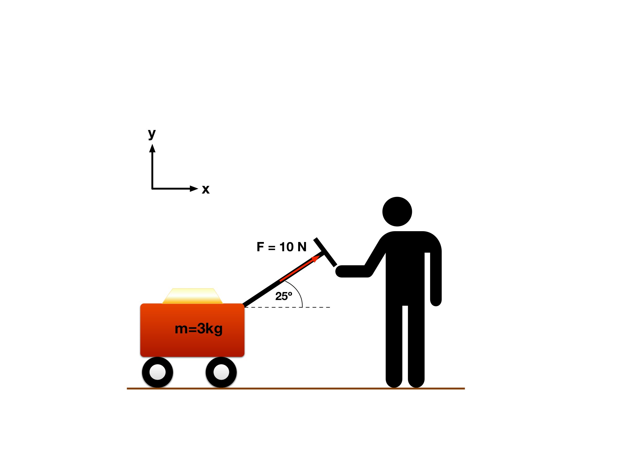
Step 1: Separate the pull into components. Take right as positive x and up as positive y. The 10 N pull has components 10 cos 25° to the right and 10 sin 25° upward.
The problem models the cart as sliding right with μₖ = 0.3 and no vertical acceleration. Its upward pull partly supports its weight, so the normal force is smaller than mg. The wheels in the original drawing are illustrative; use the stated sliding model.
Read every step and figure
Step 1
Step 1: Separate the pull into components. Take right as positive x and up as positive y. The 10 N pull has components 10 cos 25° to the right and 10 sin 25° upward.
The problem models the cart as sliding right with μₖ = 0.3 and no vertical acceleration. Its upward pull partly supports its weight, so the normal force is smaller than mg. The wheels in the original drawing are illustrative; use the stated sliding model.
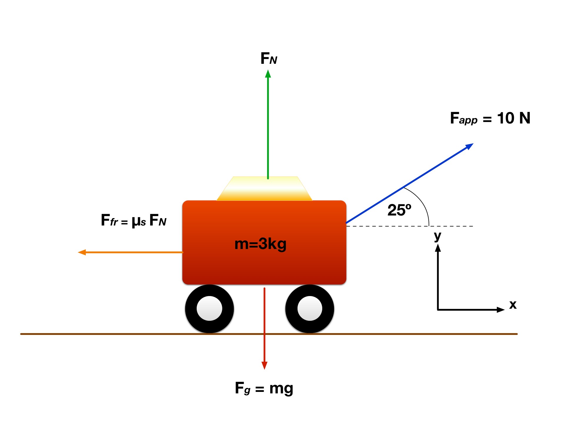
Step 2: Read the free-body diagram. Weight mg points down, the normal force N points up, the pull points up and right, and kinetic friction points left.
Correction to the retained drawing: its label Ffr = μₛ FN is not the model used here. For the stipulated sliding motion, use fₖ = μₖN with μₖ = 0.3. Static friction would satisfy 0 ≤ fₛ ≤ μₛN, reaching equality only at impending slip.
With aᵧ = 0, N = mg − 10 sin 25°. Then ΣFₓ = 10 cos 25° − μₖN = maₓ. Keep the pull’s upward component in the vertical balance! Friction model reference.
Read every step and figure
Step 1
Step 2: Read the free-body diagram. Weight mg points down, the normal force N points up, the pull points up and right, and kinetic friction points left.
Correction to the retained drawing: its label Ffr = μₛ FN is not the model used here. For the stipulated sliding motion, use fₖ = μₖN with μₖ = 0.3. Static friction would satisfy 0 ≤ fₛ ≤ μₛN, reaching equality only at impending slip.
With aᵧ = 0, N = mg − 10 sin 25°. Then ΣFₓ = 10 cos 25° − μₖN = maₓ. Keep the pull’s upward component in the vertical balance! Friction model reference.
As shown in this gallery, the only two forces acting in the x direction are the friction force () and the x-component of the applied force. In the y-direction, there are three total forces. Both normal force and y-component of the applied force in the positive y-direction, and gravitational force () acting in negative y-direction.
Step 3: Set up equations of motion
Next is to set up the equations of motion using the force equations for both the x and y components.
Using the third image we developed in the gallery and the approach we used in step 2, our equations of motion are:
X component:
Y component, using positive scalar magnitudes: 4.23 N + N − mg = maᵧ, with g = 9.81 m/s².
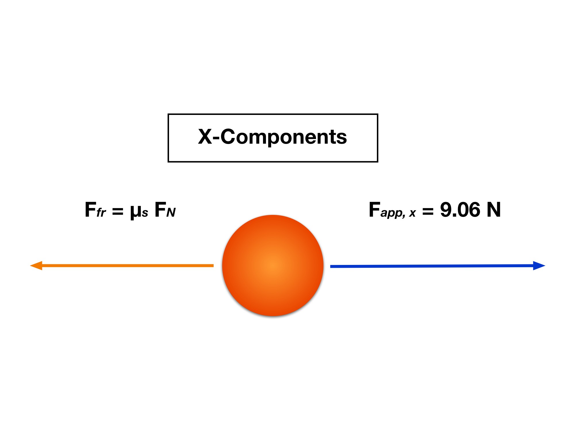
comparison of forces in the x-direction.
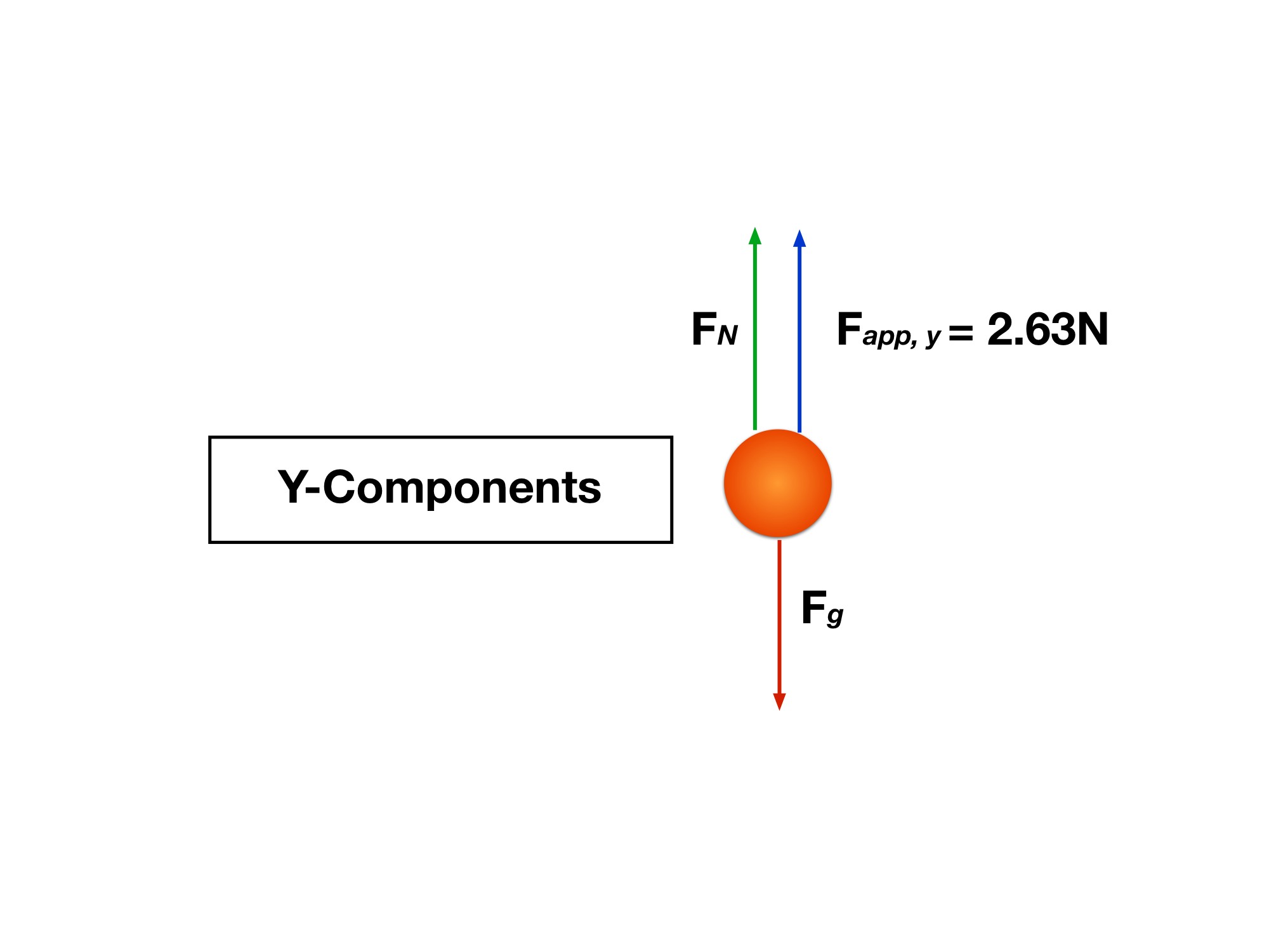
Notice here that we are subtracting the gravitational force . This is because the gravity force vector is pointing in the negative y-direction. The same with the friction force. It is being subtracted from the x-component of the applied force because it is pointed in the negative x-direction.
Step 4: Find the unknowns
Our first unknown is the normal force, .
In order to solve for , we must use our equations of motion that we prepared in step 3. We cannot use the x-component of the force, because there are two unknowns in the problem, and . We don’t know the acceleration in the x-direction.
The cart stays in contact with the horizontal surface and maintains a fixed height, so its vertical velocity remains zero and aᵧ = 0. Use the y-force balance to solve for N.
Vertical balance: 10 sin 25° + N − 3(9.81) = 0. Thus N = 29.43 − 4.22618 = 25.2038 N ≈ 25.20 N.
Step 5: Solve for the cart’s acceleration
As stated in step 4, there is no acceleration in the y-direction, so that means the cart’s acceleration is all in the x-direction. Now that we’ve solved for the normal force , and we know and , we can now solve for using the equation:
Horizontal balance: 10 cos 25° − 0.3N = 3aₓ. Substituting N = 25.2038 N gives 9.06308 − 7.56115 = 3aₓ.
aₓ = 0.500644 m/s² ≈ 0.501 m/s² to the right.
Now, after finishing that problem, you think you’re good? No, not even close! Now we will move on to a new example problem that is a little more complex, because it offers a new twist on an old classic problem.
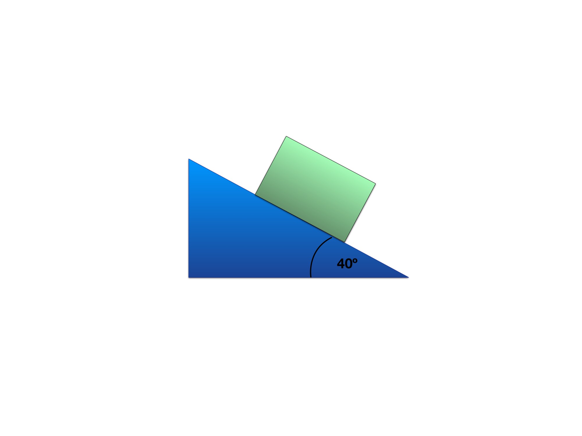
Box at rest on an inclined plane (see next image for FBD)
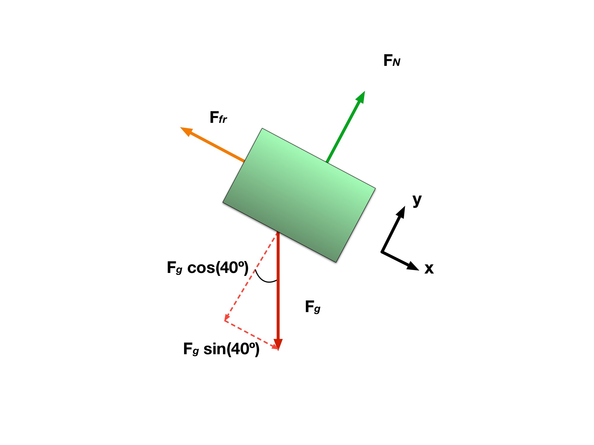
As shown in the Gallery, there is a box with a that is at rest on an inclined plane. The inclined plane creates an angle of with respect to the flat surface. Given that , determine the minimum value of the coefficient of static friction, , that is preventing the box from sliding down the plane.
Step 2: Use FBD to determine all x and y components of forces
Now that the FBD and orientation are established, we can analyze the system to separate the forces into their respective x and y components. See the gallery here to view the component forces for each direction, x and y.
Notice how the gravitational force was broken up into two separate components. The components are done to follow the reference axes, so the x and y components of the gravitational force are, respectively:
The image also shows two other forces acting on the box.
Step 4: Find the unknown normal force,
Now, we need to solve for in order to find our coefficient of static friction. How exactly are we going to do this? Well, remember in the problem statement that the box is at rest on the inclined plane. It being at rest means that it is not moving (i.e “static”).
Therefore, the box is neither accelerating in the x or y direction. Meaning then that and values are equal to ZERO.
Now our equations are:
Solving for gives us a value of .
Step 1: Set up your Free Body Diagram
Just like the previous example problem, it is imperative that an FBD is created. Look at this problem’s gallery’s second image to see the FBD. Something new to notice in the FBD is that there is no applied force acting on the box. Also notice how my reference x and y-axes are oriented differently than before. We shifted the axes’ orientations to match the orientation of the box.
Changing the orientation to that of the box’s makes the problem much easier to understand visually and it can be done for any problem where the object you are trying to analyze is in a crazy orientation!
Step 3: Set up your equations of motion (EOMs)
Let’s set up our EOMs for both the x and y components. Again we will be using both components of the force equations:
Now, using the third image in the gallery and the equations above, let’s plug in the forces for both the x and y components.
x - component:
y - component:
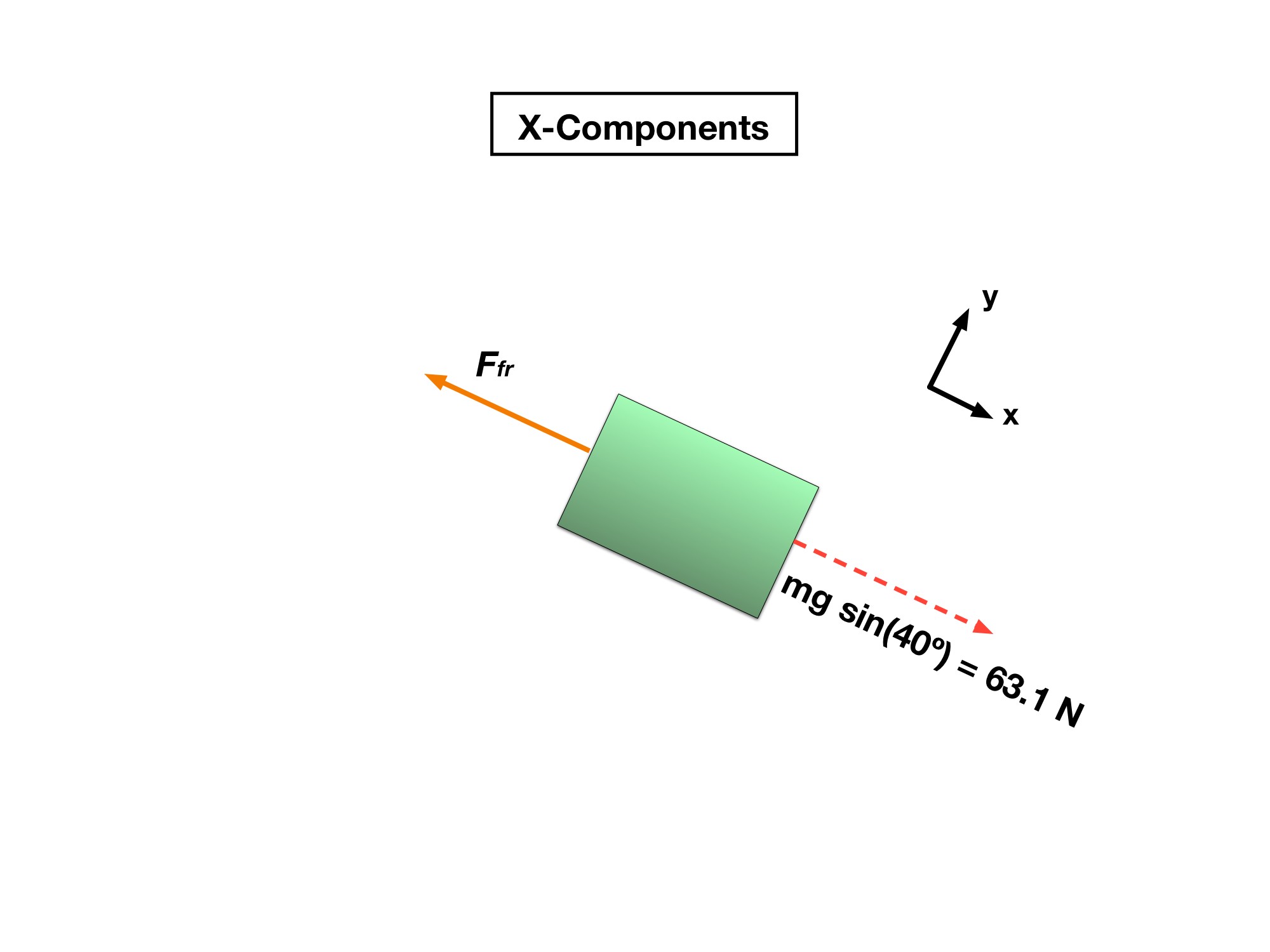
Comparison of the x-components of the problem
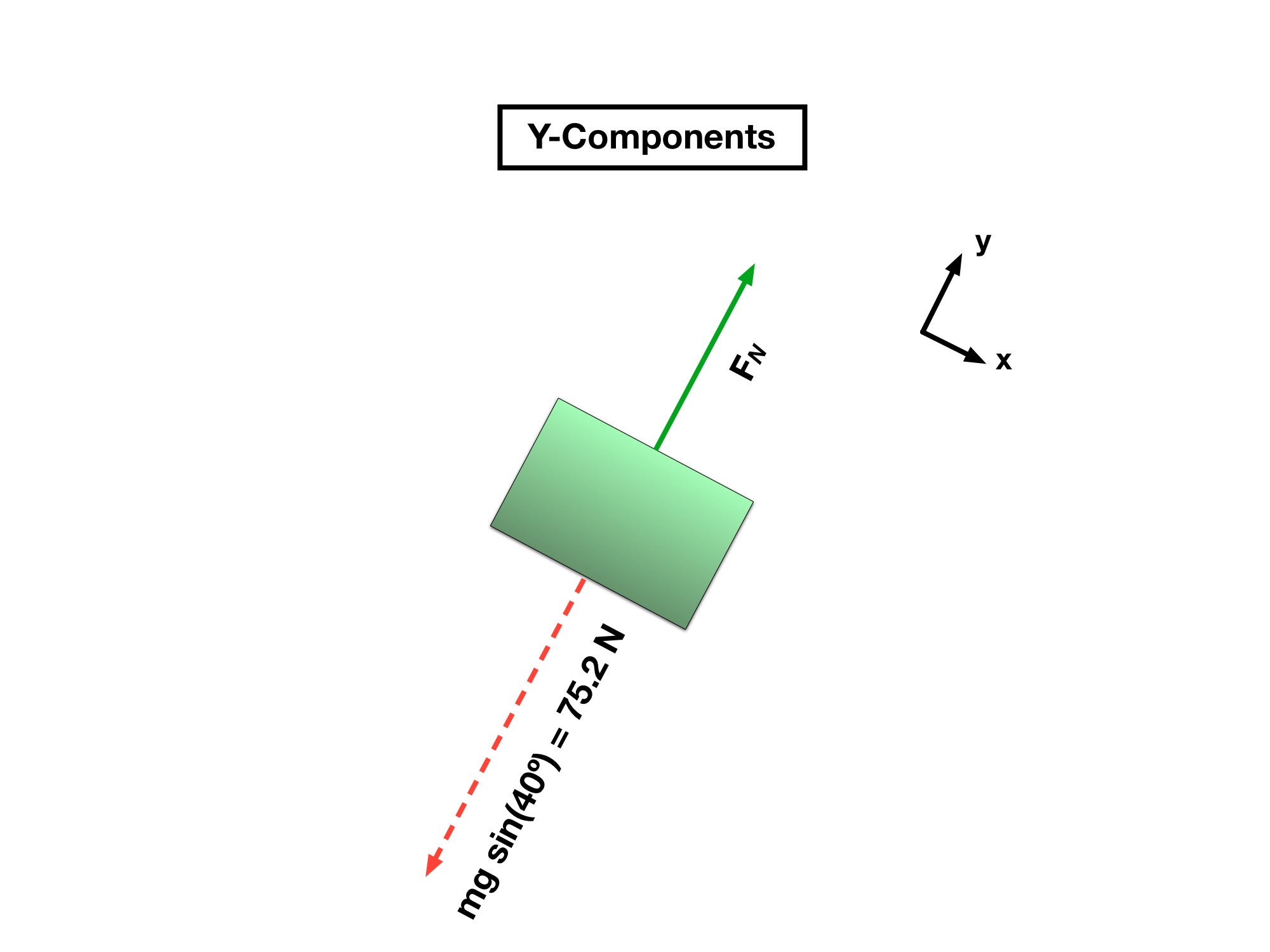
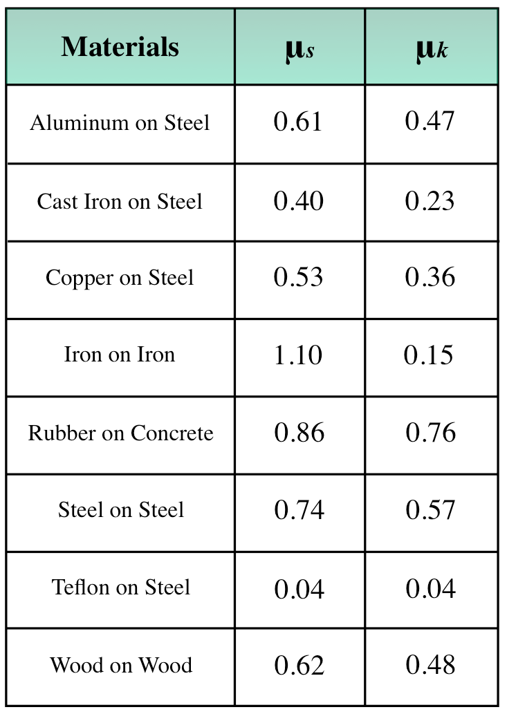
We keep saying these are high values, but what are the real coefficients like?
If you are interested in the or values for various scenarios, we have compiled a small list detailing many friction coefficients for various materials in contact with each other.
Table 1.4.1- List of Coefficient of Frictions
Pop Quiz 1.4.1 Forces as Vectors
Question 1 of 5 · 0 correct
AP Topic 2.5 · Read the worked solution
A 50 kg box remains at rest on a horizontal floor. A man pulls upward on it with 10 N. With g = 9.81 m/s², what is the normal-force magnitude?
Read every full question without answers
Question 1
Question 2
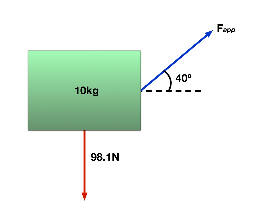
The shown 10 kg box is suspended above the ground. Only its weight (98.1 N downward) and a 5 N applied force at 40° above horizontal act on it. What is the box’s acceleration?
Question 3
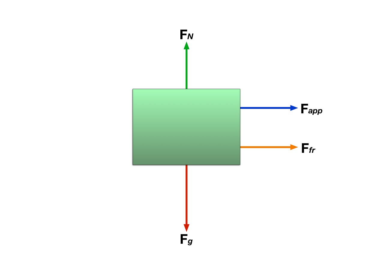
Refer to this Free Body Diagram. If the box is moving to the right, which force is incorrectly drawn?
Question 4
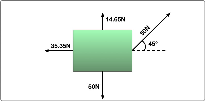
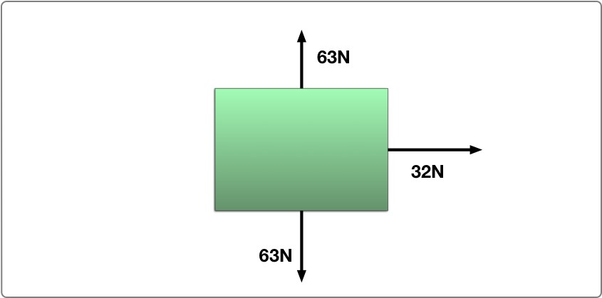
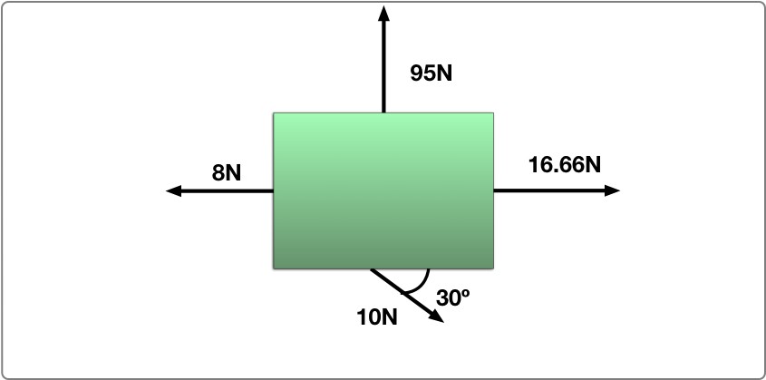
Question 5
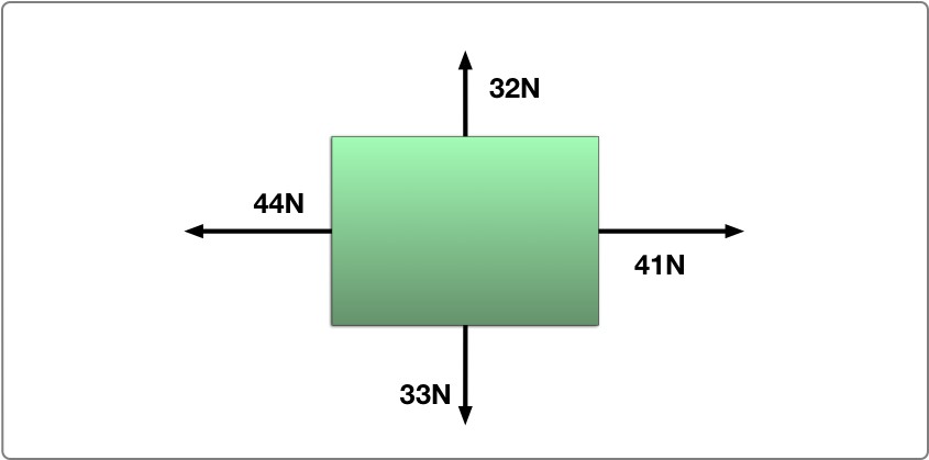
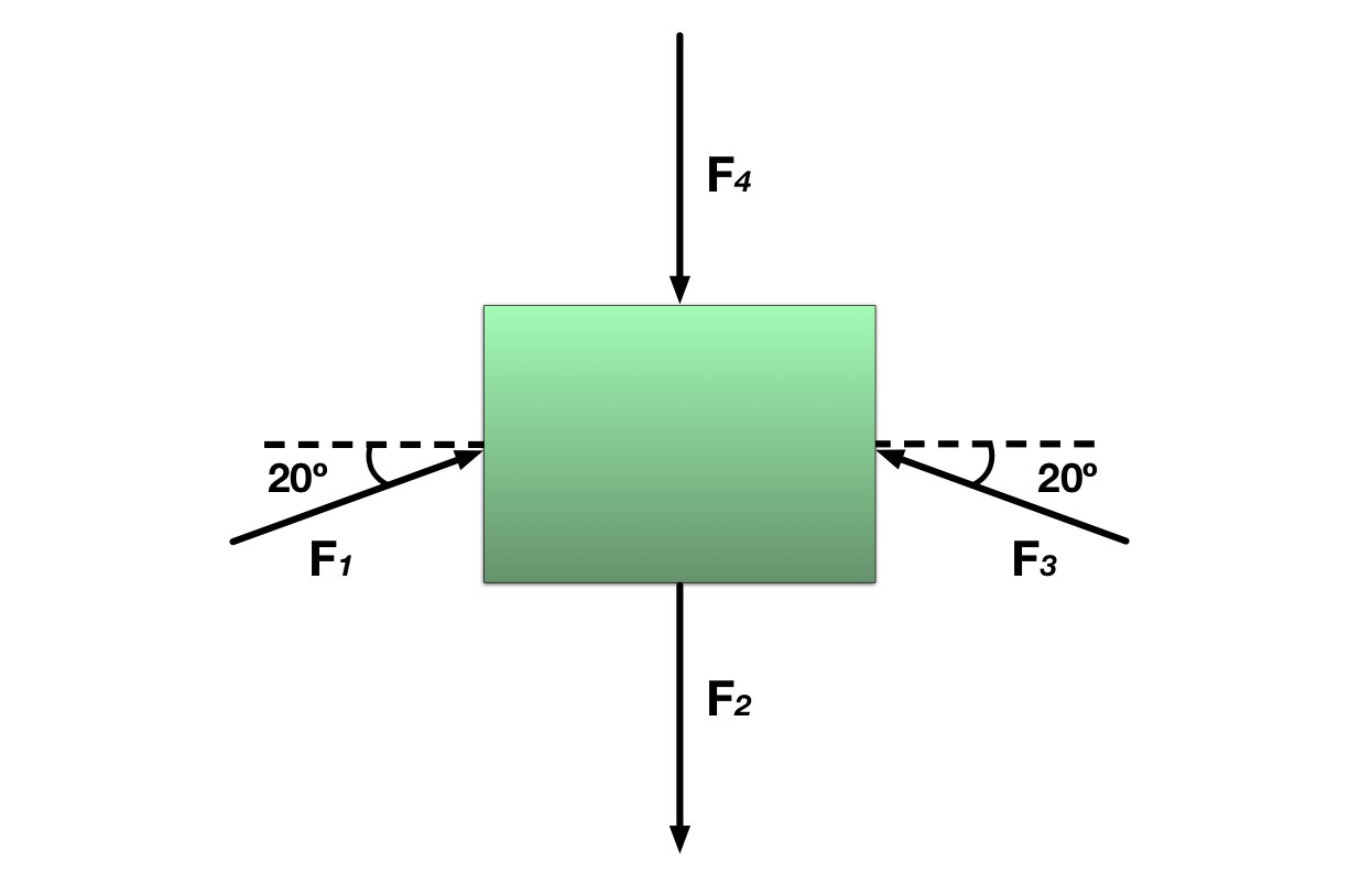
Four forces act on the same box. Each force has a magnitude of . If the box has a mass of , what is the acceleration of the box?
(Equation 1.1.1)
(Equation 1.1.2)
(Equation 1.2.1)
(Equation 1.2.2)
(Equation 1.2.3)
(Equation 1.2.4)
(Equation 1.2.5)
(Equation 1.3.1)
(Equation 1.3.2)
fₛ ≤ μₛN, with fₛ,max = μₛN at impending slip (Equation 1.4.1); ΣF⃗ = ma⃗ (Equation 1.4.2); ΣFᵧ = maᵧ (Equation 1.4.3); ΣFₓ = maₓ (Equation 1.4.4).
Original problem 2
The source answer key drops the “k” in km; use the kilometre units shown in the diagram.
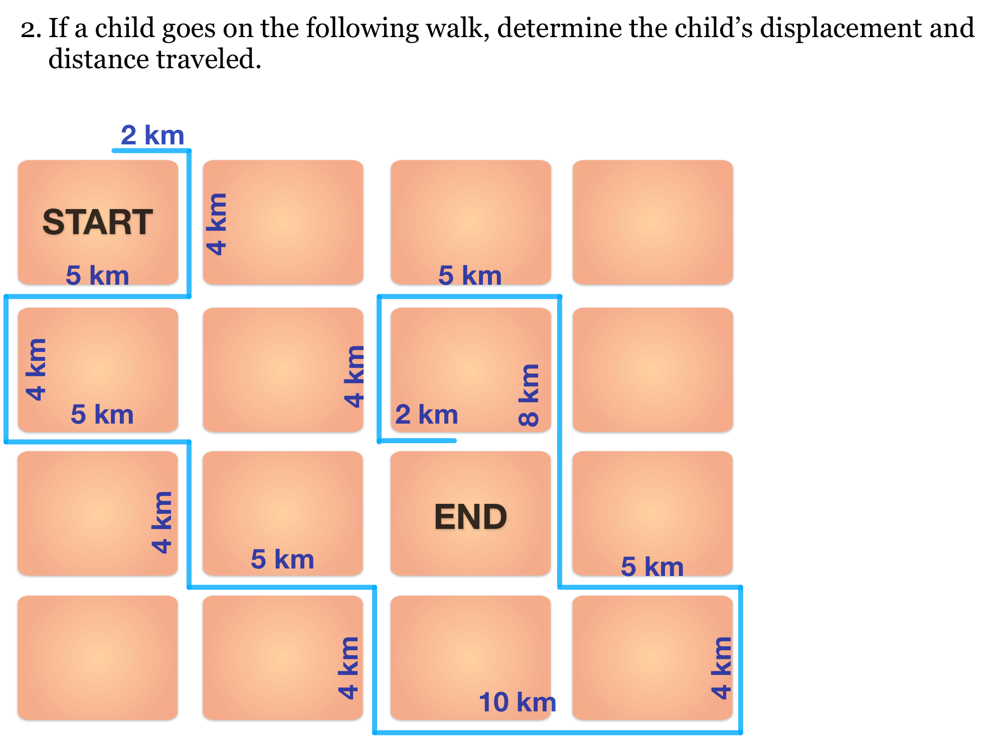
Problem text
Follow the diagram’s route. Its legs, starting at START, are: 2 km east, 4 km south, 5 km west, 4 km south, 5 km east, 4 km south, 5 km east, 4 km south, 10 km east, 4 km north, 5 km west, 8 km north, 5 km west, 4 km south and 2 km east. Find distance and displacement.
Drawing is temporarily unavailable. Work on paper if needed, then record your reasoning here.
Saving written working requires JavaScript. The problem remains available above; keep your work on paper or in your own notes.
Original problem 1
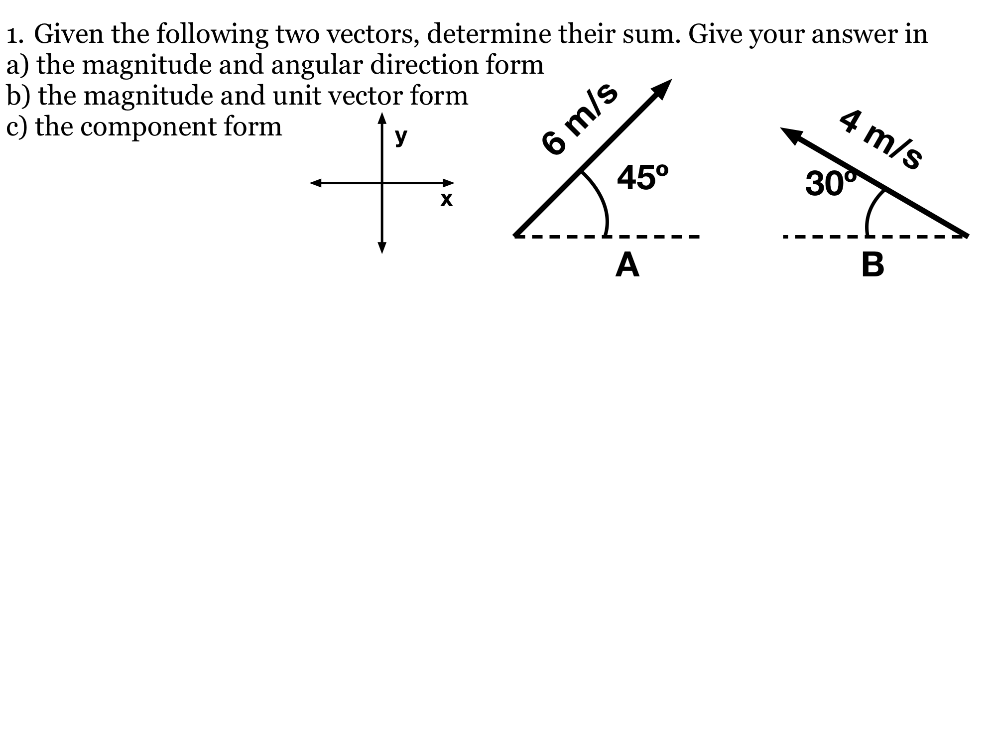
Problem text
Add A, 6 m/s at 45° counterclockwise from +x, and B, 4 m/s at 150° from +x (30° north of west). Give the result as magnitude and direction, magnitude times a unit vector, and components.
Drawing is temporarily unavailable. Work on paper if needed, then record your reasoning here.
Saving written working requires JavaScript. The problem remains available above; keep your work on paper or in your own notes.


Original problem 3
“Where is he?” has several spherical-Earth solutions; the source key lists only the North Pole.
Problem text
A man walks 1 km south, 3 km east and 1 km north and returns to his starting point. Give a possible starting point on an ideal spherical Earth, and explain why a flat-plane model cannot produce this result.
Drawing is temporarily unavailable. Work on paper if needed, then record your reasoning here.
Saving written working requires JavaScript. The problem remains available above; keep your work on paper or in your own notes.
Original problem 4
The source key gives a length unit; the cross product here has units m².
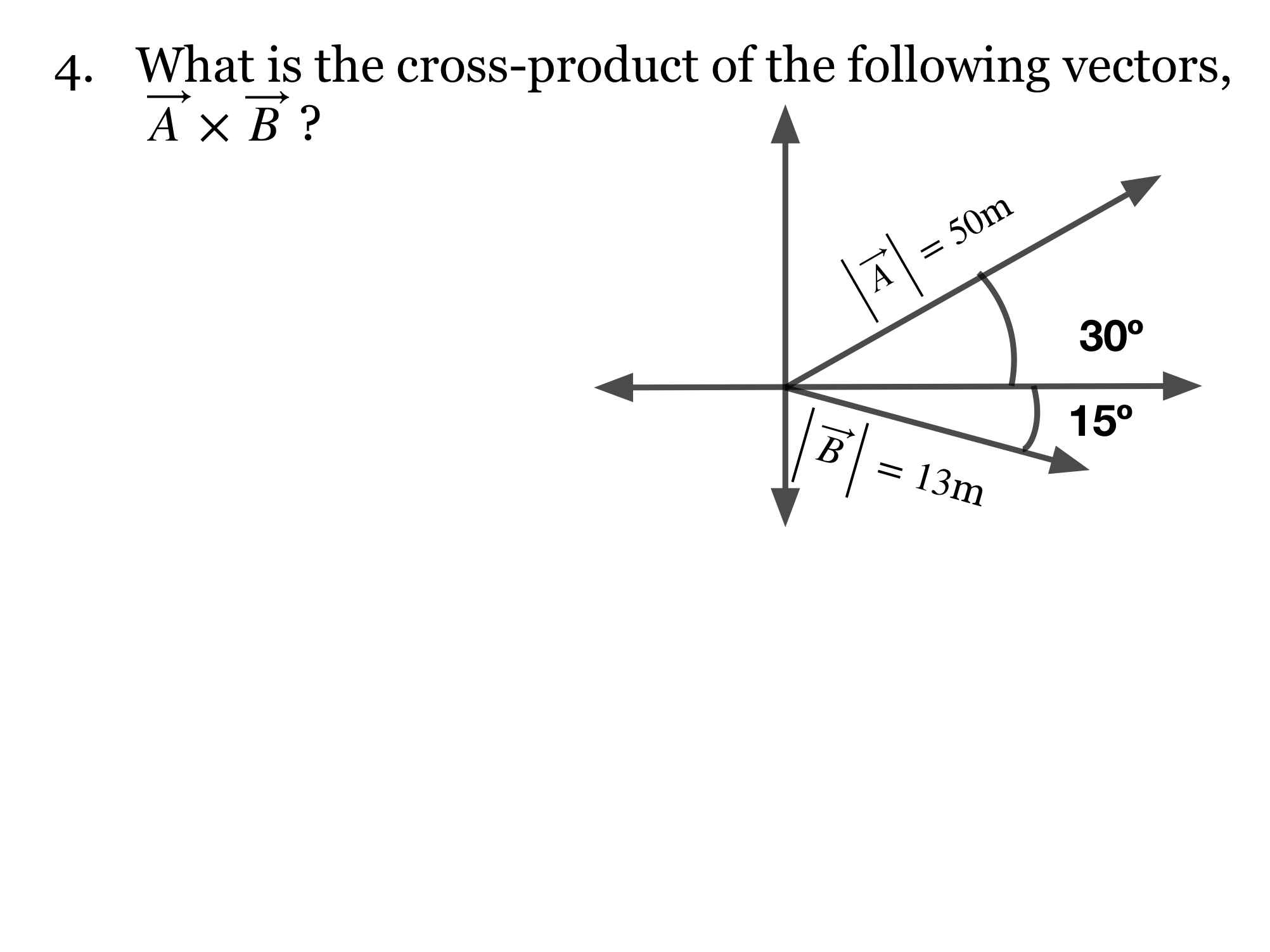
Problem text
In a right-handed x–y plane, A has magnitude 50 m and angle +30° from +x. B has magnitude 13 m and angle −15° from +x. Find A × B.
Drawing is temporarily unavailable. Work on paper if needed, then record your reasoning here.
Saving written working requires JavaScript. The problem remains available above; keep your work on paper or in your own notes.
Original problem 5
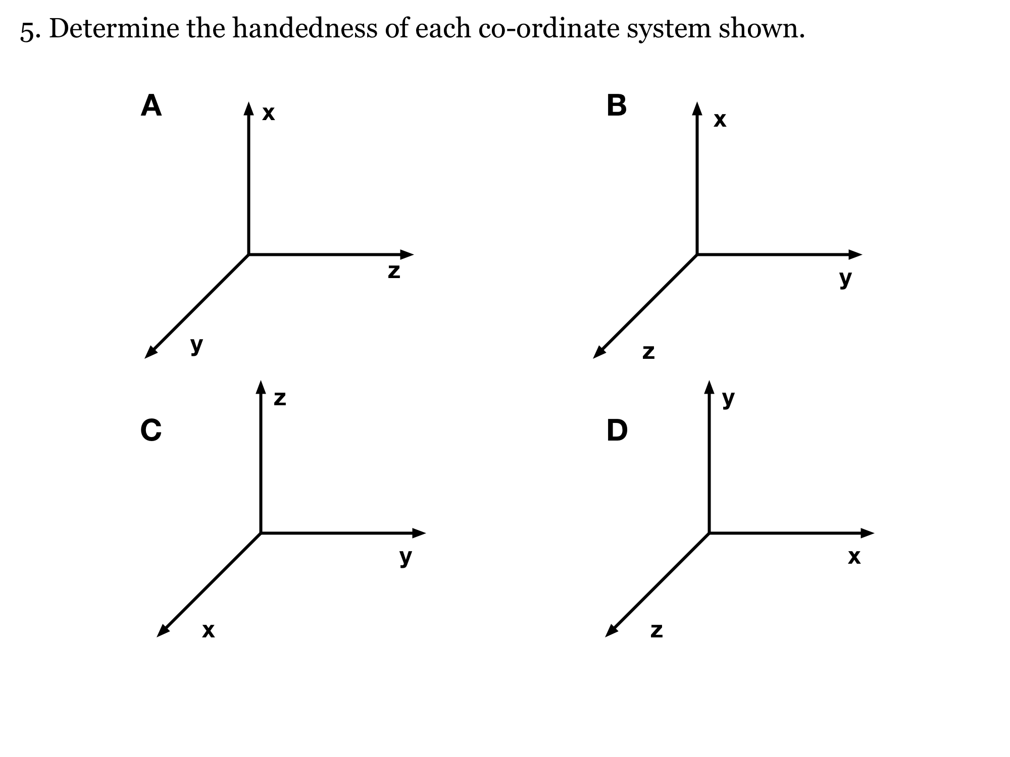
Problem text
Determine whether coordinate systems A, B, C and D in the diagram are right- or left-handed. For the perspective drawing, the diagonal axis points out toward the viewer.
Drawing is temporarily unavailable. Work on paper if needed, then record your reasoning here.
Saving written working requires JavaScript. The problem remains available above; keep your work on paper or in your own notes.
Original problem 6
This is a dot product of two forces, so its unit is N²; it is not work.
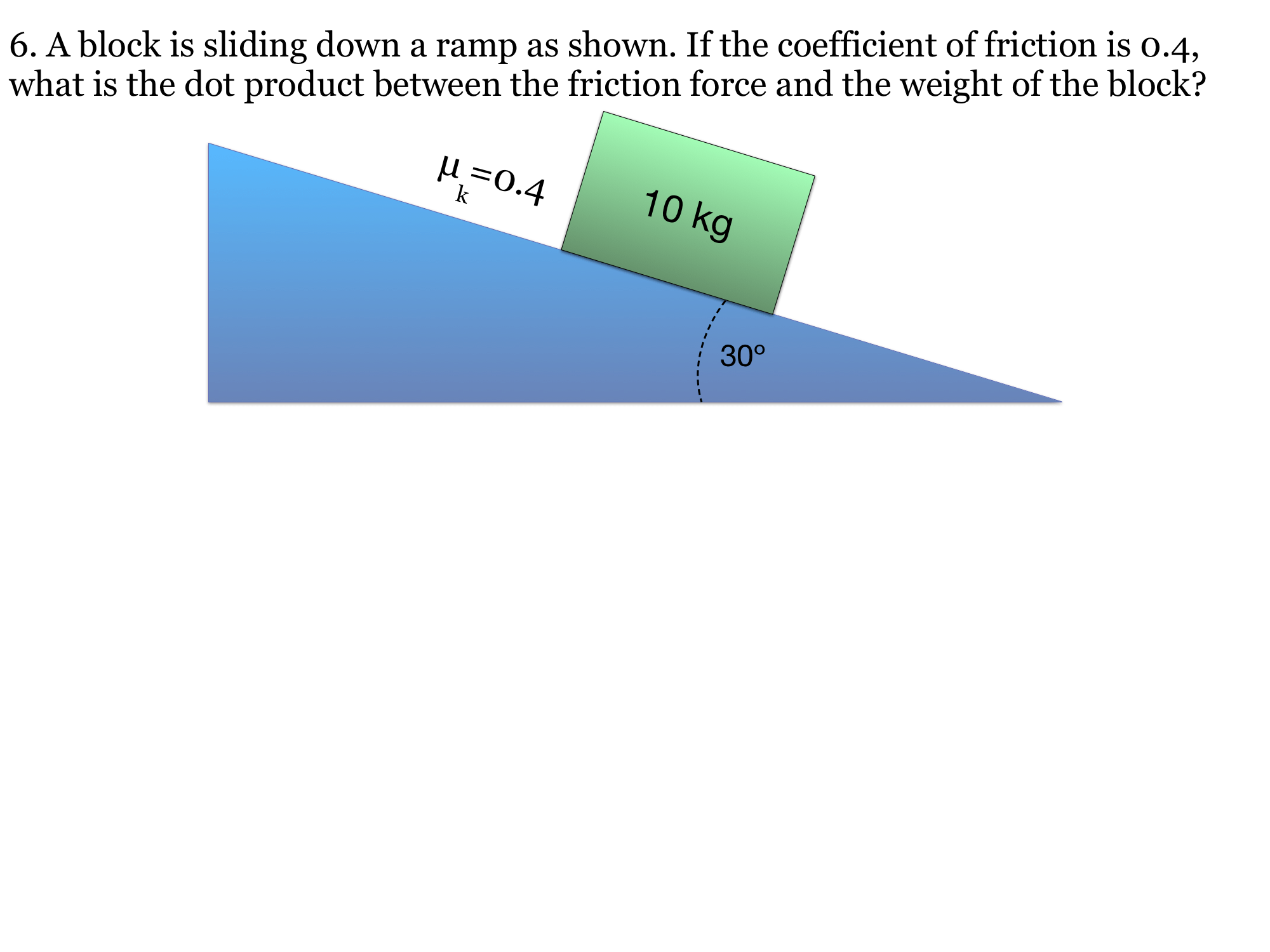
Problem text
A 10 kg block slides down a 30° ramp. The kinetic friction coefficient is 0.4. Find the dot product of the friction force and the weight. Use g = 9.8 m/s².
Drawing is temporarily unavailable. Work on paper if needed, then record your reasoning here.
Saving written working requires JavaScript. The problem remains available above; keep your work on paper or in your own notes.
Original problem 7
The source’s unconditional answer overlooks the zero-vector case.
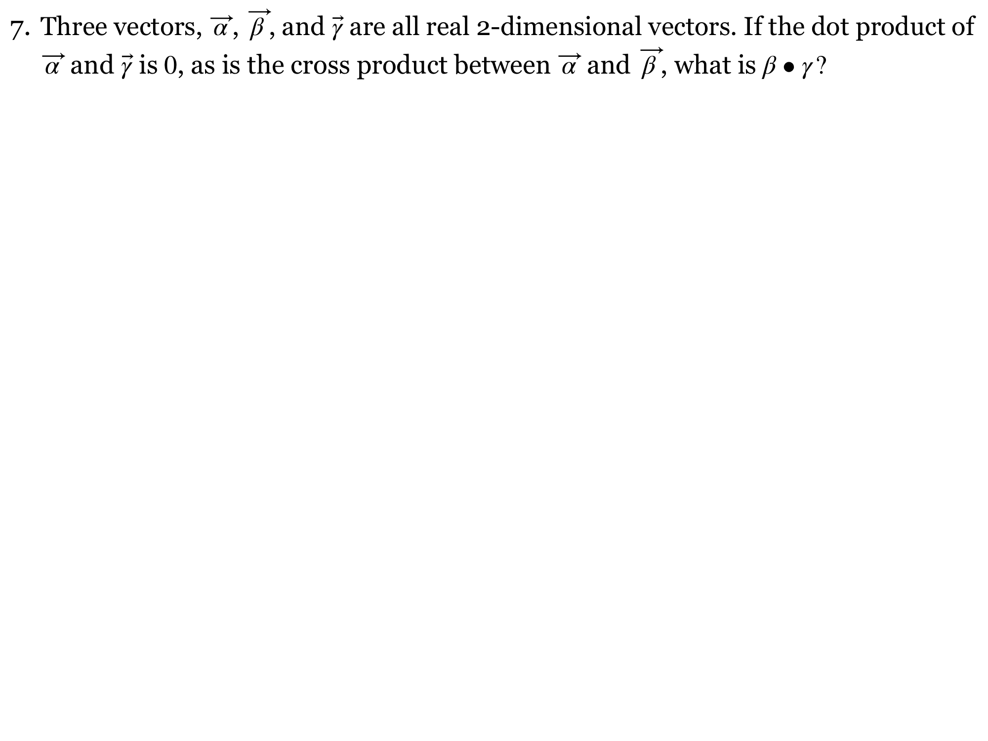
Problem text
For real two-dimensional vectors α, β and γ, α · γ = 0 and α × β = 0. What can you conclude about β · γ? Consider separately α ≠ 0 and α = 0.
Drawing is temporarily unavailable. Work on paper if needed, then record your reasoning here.
Saving written working requires JavaScript. The problem remains available above; keep your work on paper or in your own notes.
Original problem 8
Use the magnitude of displacement in this scalar ratio; a vector divided by distance would remain a vector.
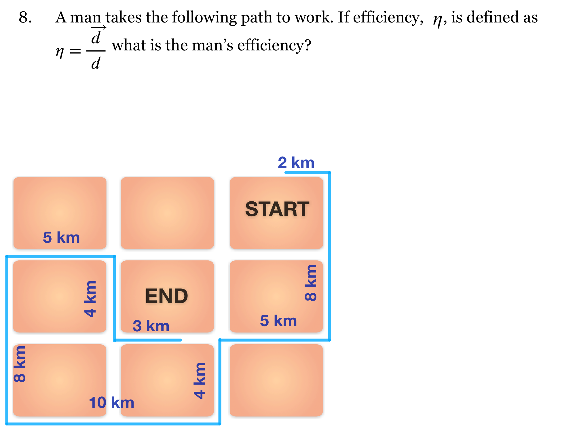
Problem text
Use the pictured path: 2 km east, 8 km south, 5 km west, 4 km south, 10 km west, 8 km north, 5 km east, 4 km south and 3 km east. Define route efficiency as η = |displacement| / distance traveled. Find η.
Drawing is temporarily unavailable. Work on paper if needed, then record your reasoning here.
Saving written working requires JavaScript. The problem remains available above; keep your work on paper or in your own notes.
Original problem 9
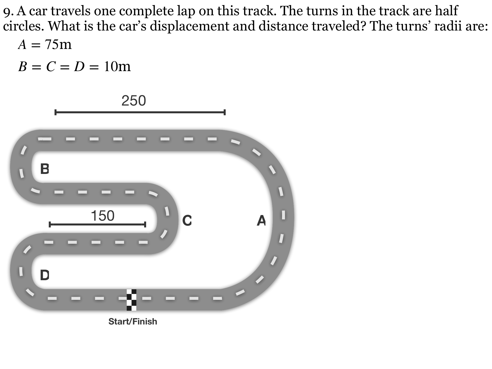
The original A = 75 m cannot connect the depicted three 10 m semicircles with horizontal straights: vertical closure requires 2RA = 2(RB + RC + RD). This reviewed version repairs A to 30 m. Taking the original arc radii independently would give 1129.87 m, but that geometry would not close.
Problem text
The diagram is a closed track with four semicircular turns. Correct radius A to 30 m; retain B = C = D = 10 m. The two outer straight segments are each 250 m and the two inner straight segments are each 150 m. Find displacement and distance for one complete lap.
Drawing is temporarily unavailable. Work on paper if needed, then record your reasoning here.
Saving written working requires JavaScript. The problem remains available above; keep your work on paper or in your own notes.
Original problem 10
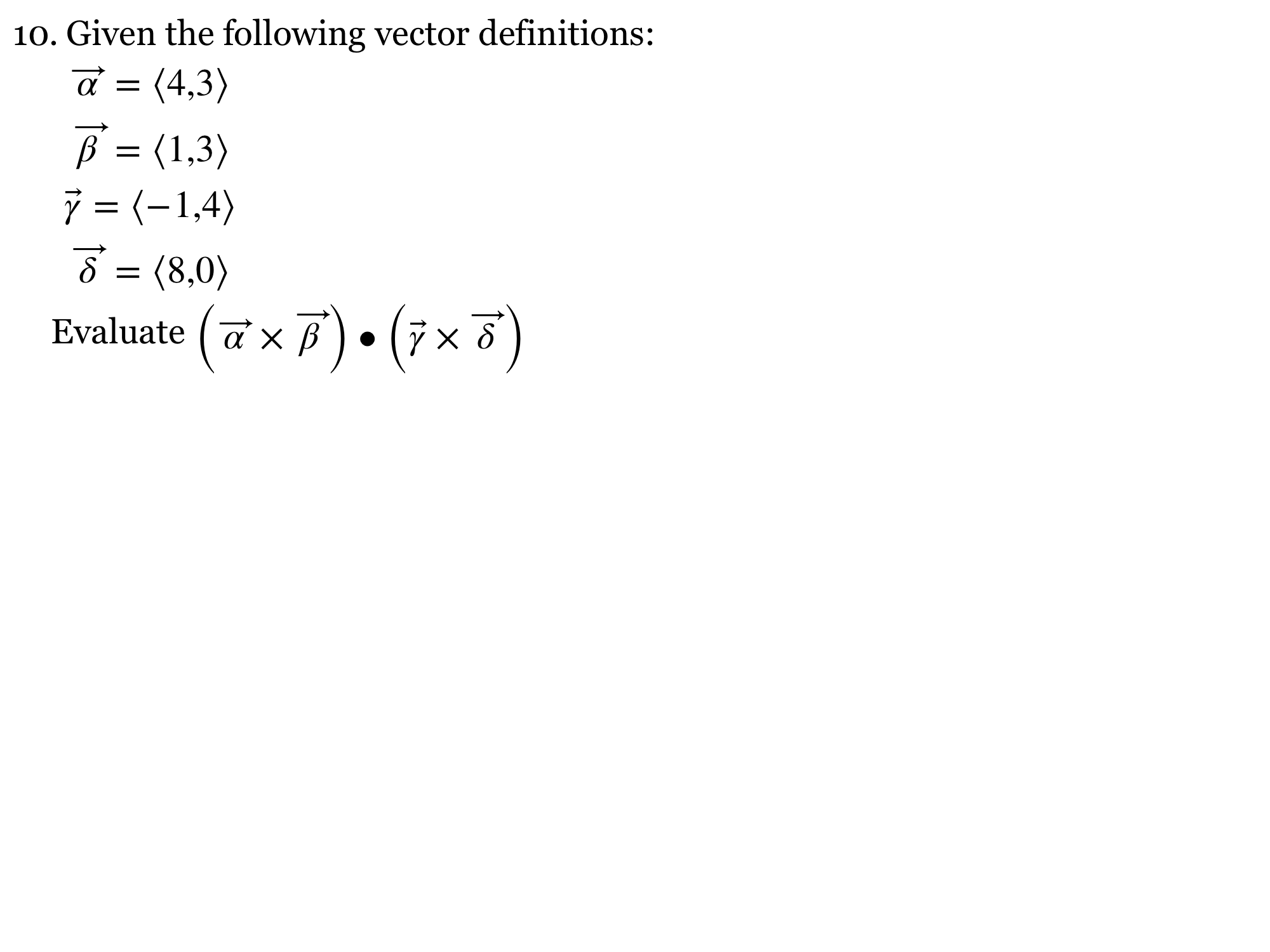
Direct component calculation corrects the source key’s −387.6.
Problem text
Embed the following vectors in the x–y plane of a right-handed 3D system: α = (4, 3), β = (1, 3), γ = (−1, 4), δ = (8, 0). Evaluate (α × β) · (γ × δ).
Drawing is temporarily unavailable. Work on paper if needed, then record your reasoning here.
Saving written working requires JavaScript. The problem remains available above; keep your work on paper or in your own notes.
Reviewed physics notes (13)
These corrections keep the original lesson’s purpose while fixing errors in the source edition.
- Friction is not generically resistance to all motion between liquids and solids. — Reference 1
- Source writes static friction as an equality and aligns it with the normal-force vector. — Reference 1
- Source subtracts already directed vectors, risking double-sign errors. — Reference 1
- Wheel rolling friction is not Coulomb sliding friction, and “just begins” concerns static rather than kinetic friction. — Reference 1
- Original combines a negative gravity vector with a subtraction, causing sign inconsistency. — Reference 1
- Zero velocity at one instant does not in general imply zero acceleration. — Reference 1
- Original presents only an equality without explaining the minimum threshold. — Reference 1
- Formula list must agree with corrected static-friction law and use scalar components. — Reference 1
- Normal force requires contact and vertical-equilibrium assumptions; native 480.5 N key is retained. — Reference 1
- Image has no normal force; clarifies free-flight assumption needed for native 9.497 m/s² answer. — Reference 1
- Keep scalar g positive and avoid truncating intermediate values. — Reference 1
- Use consistent unrounded force components. — Reference 1
- Source 0.503 m/s² results from truncated intermediate values. — Reference 1
Glossary and deeper reading · 11 refreshers
These editorial refreshers supplement the reading. Definitions and examples are added guidance; original source wording and recorded answers remain in their original context.
-
Force
A force describes an interaction that can change an object’s momentum. It is a vector measured in newtons, so both size and direction matter when forces are added. For example, a rope can pull a cart while the floor exerts friction in another direction.
-
Static friction
Static friction opposes the tendency for relative sliding between surfaces that are not sliding at their contact. In the simple model it adjusts up to a maximum set by the coefficient of static friction and normal force. For example, static friction can push a walking person forward when the foot pushes backward on the ground.
-
Kinetic friction
Kinetic friction acts between surfaces that slide relative to one another. It opposes their relative slipping and is often modeled with magnitude equal to the kinetic-friction coefficient times the normal force. For example, a rapidly moving belt can exert forward kinetic friction on a slower box sliding on it.
-
Vector
A vector is a quantity with a magnitude and a direction, represented by an arrow or by components along chosen axes. Vectors add by adding corresponding components rather than simply adding their magnitudes. For example, an eastward displacement followed by a northward displacement produces a resultant pointing northeast. The zero vector has zero magnitude and no unique direction.
-
Magnitude
Magnitude is the nonnegative size of a vector quantity. It does not specify direction, and it differs from a signed component. For example, a westward velocity can have a negative x component while its speed, the velocity magnitude, stays positive.
-
Vector component
A vector component describes the part of a vector along a chosen axis. Its signed value changes when the axes change, even though the physical vector remains the same. For example, a diagonal launch velocity can be resolved into horizontal and vertical components that share the same elapsed time.
-
Drag
Drag is a force from a fluid that opposes an object’s motion relative to that fluid. Its dependence on speed, shape, and fluid properties varies with the physical regime. For example, a parachute increases air drag by presenting a large area to the moving air.
-
Gravity
Gravity is the attractive interaction between masses in the Newtonian model. For spherical bodies or point-mass approximations, its strength decreases with the square of the separation between their centers. For example, Earth’s gravity provides the inward force that keeps a satellite in orbit.
-
Scalar
A scalar is a quantity described by a value and unit without a spatial direction. A scalar can have a sign when its definition or reference permits one; scalar does not mean always positive. For example, mass is a scalar, whereas the velocity of that mass also needs a direction.
-
Free-body diagram
A free-body diagram shows the external forces acting on one selected object or system. Each arrow names a real interaction, and its direction is the direction of that force. For example, a book resting on a desk has a downward gravitational force and an upward normal force; velocity is not an extra force arrow.
-
Acceleration
Acceleration is the vector rate of change of velocity with time. It can change an object’s speed, direction, or both, and it is measured in meters per second squared. For example, a satellite moving at constant speed in a circular orbit accelerates toward the center.