Dampened Harmonics
Original textbook reading.
Enrichment beyond the AP course.
The preceding section used ideal conservative oscillators. Real oscillators also experience dissipative forces, which remove mechanical energy and reduce the amplitude. This section models linear viscous damping.
Dampened Harmonics
Figure 10.3.1 Ball String Harmonics...Dampening?
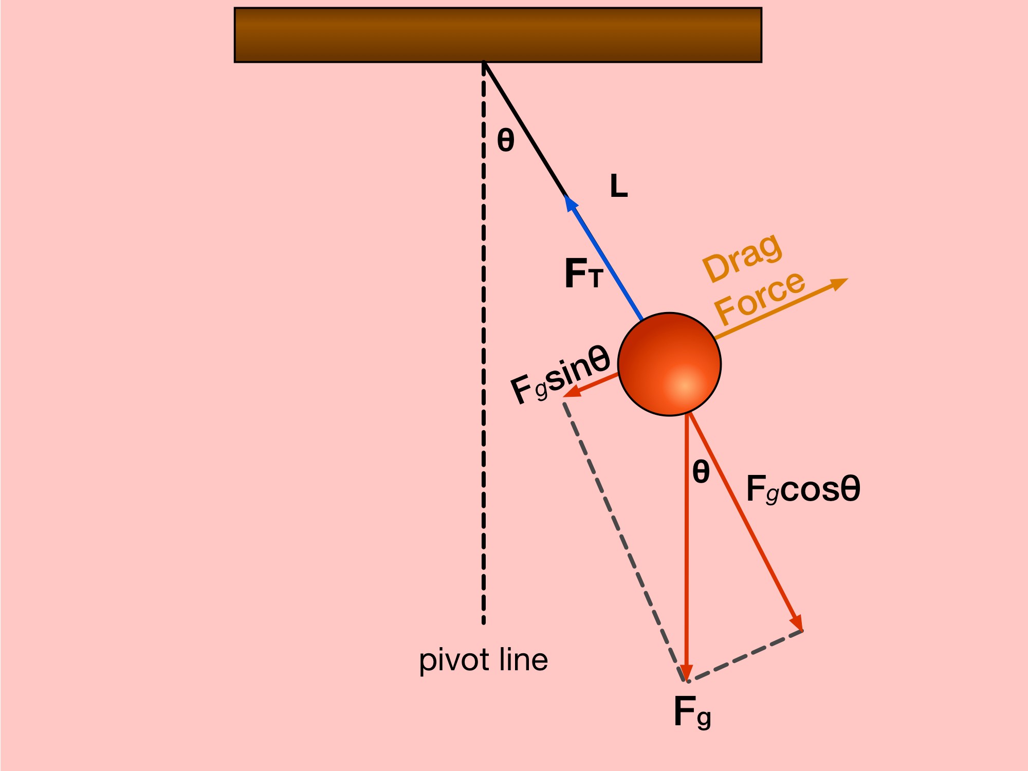
For the ideal pendulum, gravity and tension act while air drag and pivot friction are neglected. Small-angle motion is then approximately harmonic and its amplitude is constant.
In reality though, the ball is subjected to an external force when suspended in the air called drag force. Remember that drag force we can think of as air resistance that an object feels. This drag force is the reason that the ball slows down and eventually stops.
A force that dissipates mechanical energy damps an oscillator. In the linear viscous model the resistive force is proportional to velocity and opposite its direction: F_d=−bẏ. The coefficient b has units kg/s.
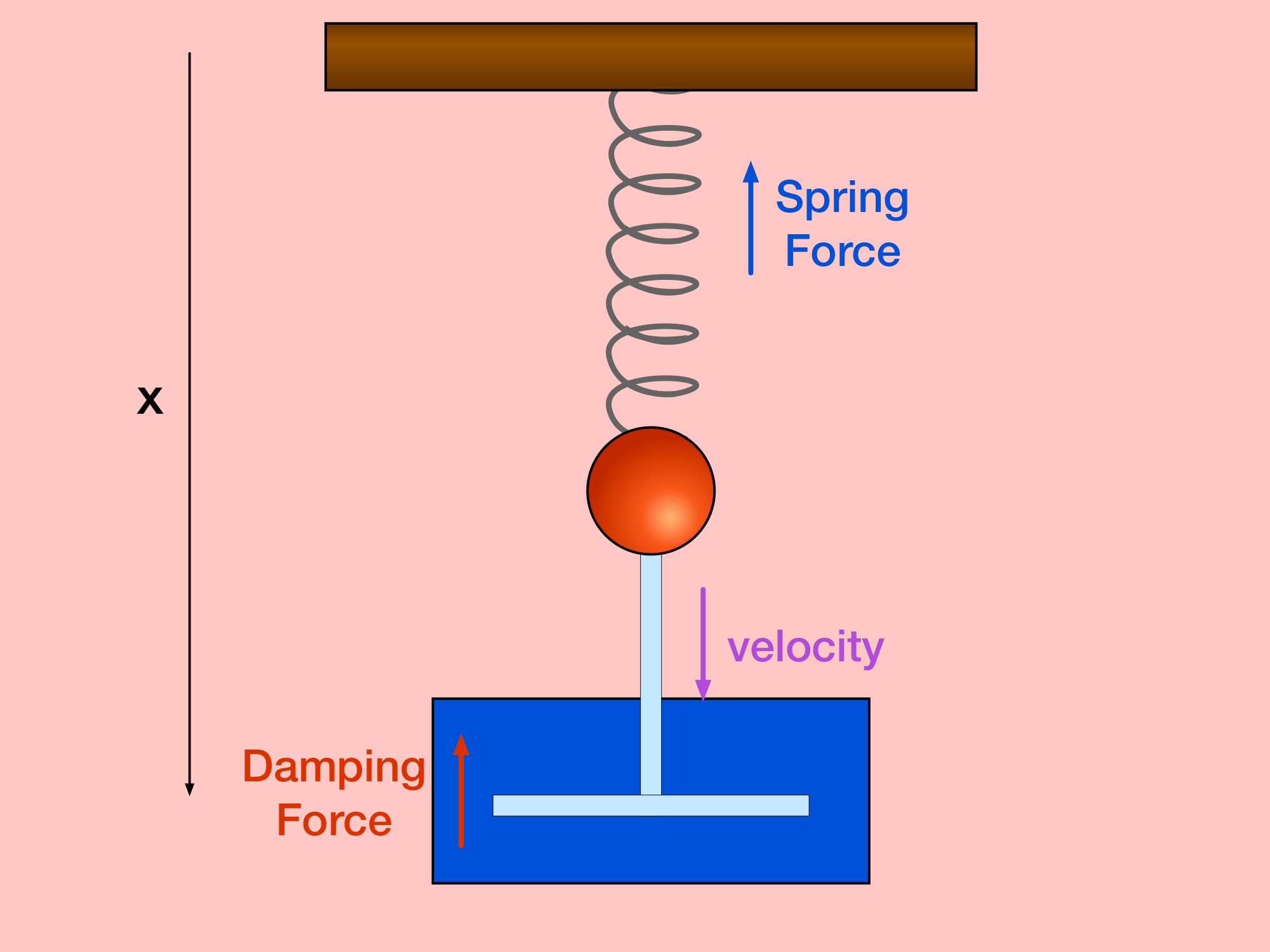
For the illustrated spring and immersed plate, approximate the water’s resistive force as F_d=−bẏ. Measure displacement from static equilibrium and use the total moving mass m. Then mÿ+bẏ+ky=0. For b<2√(mk), the motion is underdamped and its amplitude envelope decays exponentially.
Figure 10.3.2 Classic Dampened Harmonics
The equation that we will be using is:
Here y(t) is displacement from equilibrium, A₀ is the envelope coefficient at t=0, b is the damping coefficient in kg/s, ω_d is the damped angular frequency in rad/s, m is the moving mass and α is a phase in radians. In general y(0)=A₀cosα, not A₀.
The angular frequency is equal to:
The undamped natural frequency is ω₀=√(k/m). Linear damping gives ω_d²=ω₀²−[b/(2m)]². If b=0 the model reduces to SHM. At b=2√(mk) it is critically damped, and for larger b it is overdamped; these two cases do not have an oscillation period.
Figure 10.3.3 Graphed Example of Dampened Harmonics
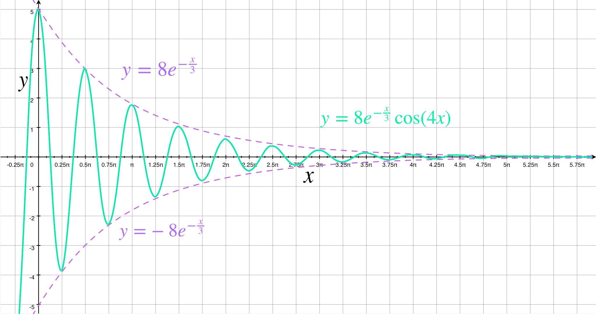
A lot to handle... I know, but hopefully the graphs that follow will give you a better understanding.
The exponential curves bound the oscillatory displacement. Their values approach zero as time grows; they do not reach zero at a finite time in this ideal viscous model. Real instruments may report rest once motion is below a detection threshold.
Figure 10.3.4 A More Dramatic Example of Dampened Harmonics
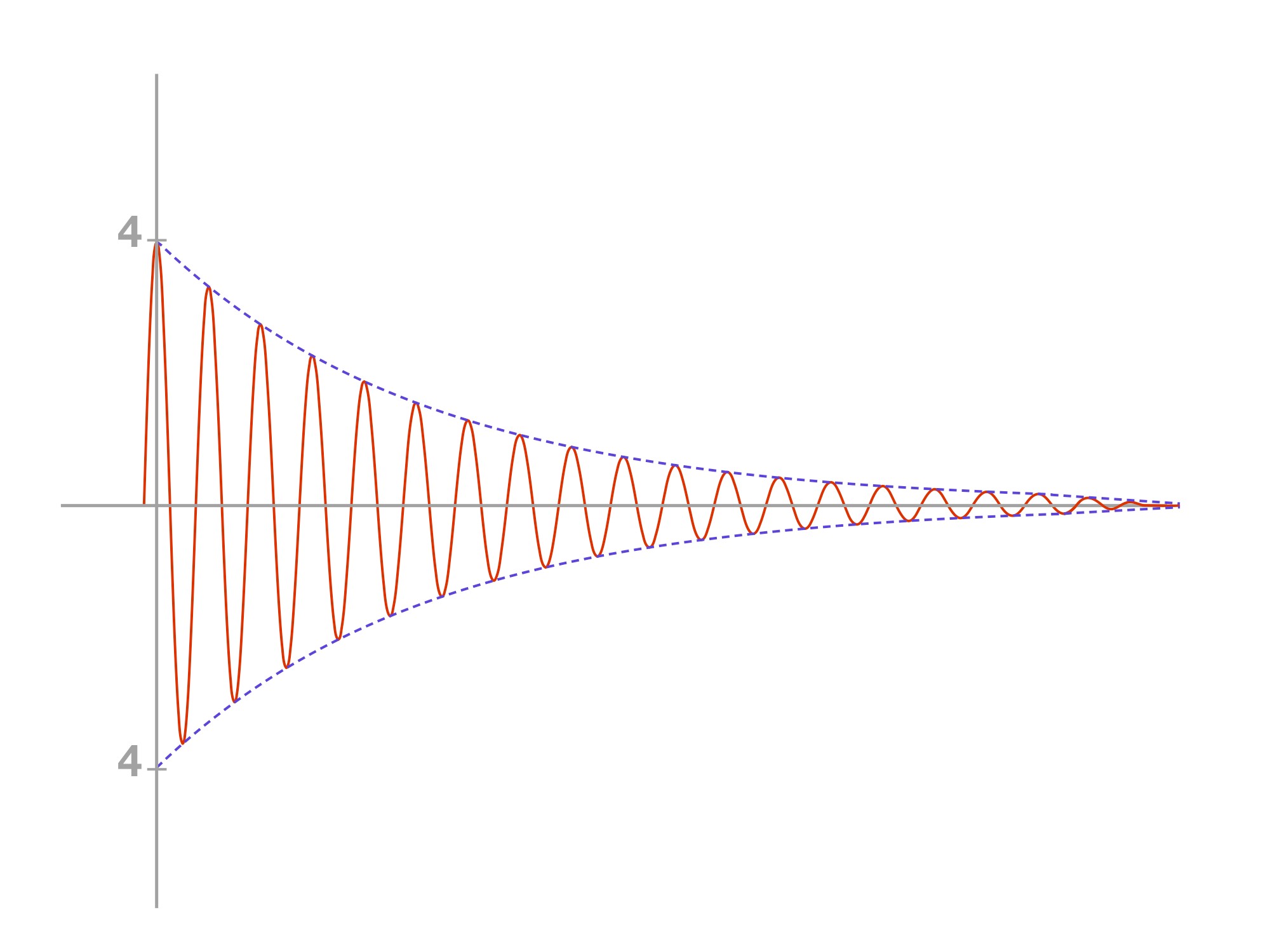
The image below is another example of how dampening effects can be much more crazy looking. In this case, the angular frequency is very high, which is why the distances between each crest is shorter than from the first image.
Example Problem 10.3.1
Lets use the ball and spring to model our example question. If the ball has a mass of , the spring a value of and value of what is the period of the motion of our ball and how long does it take for the amplitude to drop to a quarter of it’s initial value?
Example Problem 10.3.1
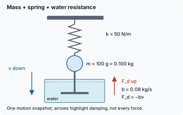
The diagram uses the same k = 50 N/m, m = 0.100 kg and b = 0.08 kg/s as the worked example. The original conflicting 90 N/m label has been replaced. This is an apparatus sketch with a damping-force highlight, not a complete FBD. Damped-oscillation model.
Step 1: Make the problem Easier
Compare quantities with matching dimensions: the decay rate is β=b/(2m)=0.400 s⁻¹, while ω₀=√(k/m)=√500=22.3607 rad/s. Their dimensionless ratio is β/ω₀≈0.0179, so the frequency correction is small. Damping still controls the amplitude decay.
Step 2: Solve for the period of the motion
Use the damped period T_d=2π/ω_d. For weak damping it is close to the undamped mass–spring period T₀=2π√(m/k).
T_d=2π/√[k/m−(b/(2m))²].
Plug in our known values to get:
T_d=2π/√[(50 N/m)/(0.100 kg)−((0.080 kg/s)/(2×0.100 kg))²].
T_d=0.281038 s≈0.28 s; T₀=0.280993 s, so the rounded result is unchanged.
Step 3: Find the amplitude of the original function
Now this seems like it’s hard because we don’t have an original displacement function representing the oscillation nor do we have a graph to interpret.
But this is a lot easier than you think. Remember our equation for dampened harmonics:
y(t)=A₀e^(−bt/(2m))cos(ω_d t−α).
The amplitude envelope, distinct from the instantaneous displacement, is A(t)=A₀e^(−bt/(2m)).
The independent variable is time. The displacement is:
y(t)=A₀e^(−bt/(2m))cos(ω_d t−α).
Notice then if you were to replace with a value of zero. This would then reduce to:
At t=0, the exponential factor is 1, so y(0)=A₀cosα.
A(0)=A₀, whereas y(0)=A₀cosα.
A₀ is the largest envelope value for t≥0. The instantaneous displacement need not attain that value when its phase is arbitrary.
Step 4: Find the value of such that the amplitude is of original amplitude
Now that we know our max amplitude, and since we know that the amplitude at any time, can be represented by the first part of our


Reviewed physics notes (44)
These corrections keep the original lesson’s purpose while fixing errors in the source edition.
- External forces in general need not cause damping. — Reference 1
- An undamped pendulum still has external forces and only small-angle SHM. — Reference 1, Reference 2
- Define damping by dissipation rather than any external force. — Reference 1
- Identify the model and its regime without promising a finite stopping time. — Reference 1
- The independent variable is time and the decay exponent is dimensionless. — Reference 1
- The amplitude envelope coefficient is not generally the initial displacement. — Reference 1
- State the underdamped validity condition. — Reference 1
- The cosine solution is not valid as an oscillation for every damping strength. — Reference 1
- Avoid confusing asymptotic decay with exact finite stopping. — Reference 1
- Comparing numerical b and k directly is dimensionally invalid; small damping does not mean no effect. — Reference 1
- A spring oscillator is not a normal pendulum, and the exact damped period is available. — Reference 1
- Use the damped period formula. — Reference 1
- Retain the small but nonzero frequency correction. — Reference 1
- Calculate and compare rather than discarding damping by a dimensional comparison. — Reference 1
- Use time consistently. — Reference 1
- Avoid an unnecessary spatial-to-temporal variable substitution. — Reference 1
- Use the physical independent variable consistently. — Reference 1
- Use consistent symbols. — Reference 1
- The cosine phase cannot be dropped. — Reference 1
- Distinguish initial envelope from initial displacement. — Reference 1
- Correct the unrestricted initial maximum claim. — Reference 1
- Amplitude decay is not a continual decrease of oscillation frequency. — Reference 1
- Avoid finite-time exact-rest inference. — Reference 1
- The envelope and zero crossings describe different things. — Reference 1
- A graph’s visual resolution cannot establish exact rest. — Reference 1
- Separate frequency, envelope decay and instantaneous crossings. — Reference 1
- Correct the misleading finite-stop title. — Reference 1
- SHM requires a restoring force; no-external-force language is inaccurate. — Reference 1, Reference 2
- The magnitude is not determined by the damping coefficient alone. — Reference 1
- Use temporal displacement and distinguish damped frequency from natural frequency. — Reference 1
- Give angular-frequency answer choices their units. — Reference 1
- Use time and the model needed to infer stiffness. — Reference 1
- Avoid leaving the inconsistent spatial equation in the second prompt paragraph. — Reference 1
- The source asked for b without supplying a mass; determine the inferable decay rate instead of fabricating m=1 kg. — Reference 1
- An evaluation time cannot determine the constant damping coefficient. — Reference 1
- These are decay-rate choices, not damping coefficients in kg/s. — Reference 1
- An arbitrary external force does not decide SHM; the repaired False statement specifically concerns nonzero viscous damping. — Reference 1
- Replace unfinished placeholder choice with a distractor. — Reference 1
- Use a consistent amplitude-envelope symbol in the calculation. — Reference 1
- Keep the envelope computation independent of the unknown phase. — Reference 1
- The source key 1/3 kg/s assumes an unstated mass. For the repaired inferable decay rate, 1/6 s⁻¹ is correct. — Reference 1
- The exponent directly identifies β=1/6 s⁻¹; no mass assumption is needed. — Reference 1
- The exact damped period is 2π/√(100−0.002²)=0.62831854 s, which rounds to 0.63 s, not 1.2 s. — Reference 1
- The 0.63 s choice matches the correct damped-period calculation. — Reference 1
Glossary and deeper reading · 14 refreshers
These editorial refreshers supplement the reading. Definitions and examples are added guidance; original source wording and recorded answers remain in their original context.
-
Mechanical energy
Mechanical energy is the sum of the kinetic and potential energies included in a model. It stays constant when transfers to or from other energy stores and across the chosen boundary are absent. For example, a pendulum’s mechanical energy can remain approximately constant while energy shifts between motion and gravitational configuration.
-
Amplitude
Amplitude is the maximum magnitude of a repeating disturbance measured from its equilibrium value. It describes the size of the oscillation rather than its frequency or propagation speed. For example, pulling a spring-mounted mass farther from equilibrium increases its oscillation amplitude when it is released from rest.
-
Pendulum
A pendulum is a system that swings about a support under a restoring torque. A simple pendulum approximates a small mass on a light string and follows simple harmonic motion only for sufficiently small angles. For example, a short string pendulum completes small swings more quickly than a longer one under the same gravitational field.
-
Gravity
Gravity is the attractive interaction between masses in the Newtonian model. For spherical bodies or point-mass approximations, its strength decreases with the square of the separation between their centers. For example, Earth’s gravity provides the inward force that keeps a satellite in orbit.
-
External force
An external force is exerted on part of a chosen system by something outside that system. The sum of external forces determines the rate of change of the system’s total momentum. For example, Earth’s gravitational force is external to a system consisting only of a falling ball.
-
Drag
Drag is a force from a fluid that opposes an object’s motion relative to that fluid. Its dependence on speed, shape, and fluid properties varies with the physical regime. For example, a parachute increases air drag by presenting a large area to the moving air.
-
Viscosity
Viscosity measures a fluid’s resistance to relative motion between neighboring layers. Viscous effects can dissipate mechanical energy and alter the velocity profile of flowing fluid. For example, honey flows more reluctantly than water under comparable conditions because it is more viscous.
-
Velocity
Velocity describes how position changes with time and includes direction. Instantaneous velocity describes one moment, while average velocity is displacement divided by elapsed time. For example, a car turning a corner can change velocity while maintaining the same speed.
-
Force
A force describes an interaction that can change an object’s momentum. It is a vector measured in newtons, so both size and direction matter when forces are added. For example, a rope can pull a cart while the floor exerts friction in another direction.
-
Displacement
Displacement is the vector change in position from the start of an interval to its end. It depends on those endpoints rather than the length or shape of the path traveled. For example, walking around a closed track and returning to the start gives zero displacement but a nonzero distance traveled.
-
Damping
Damping is a process that transfers energy out of an oscillation and reduces its amplitude over time. The motion can remain oscillatory or approach equilibrium without oscillating, depending on the damping strength. For example, an oscillator moving through a viscous liquid loses mechanical energy to the liquid.
-
Angular frequency
Angular frequency measures how rapidly the phase of a sinusoidal oscillation advances. It equals two pi times the ordinary frequency and is measured in radians per second. For example, two oscillators at the same ordinary frequency also have the same angular frequency even if their amplitudes differ.
-
Frequency
Frequency is the number of complete repeating cycles per unit time. It is measured in hertz, meaning cycles per second, and is the reciprocal of the period. For example, a vibrating string with a higher frequency produces more cycles each second.
-
Simple harmonic motion
Simple harmonic motion occurs when the net restoring force is proportional to displacement from equilibrium and points in the opposite direction. The resulting position varies sinusoidally with time in the ideal model. For example, a mass attached to an ideal spring can execute simple harmonic motion when damping is negligible.