FFR - Complex Harmonics
Original textbook reading.
Enrichment beyond the AP course.
Simple Harmonic Motion↗ is nice and all, but it’s still simple. Harmonic motion can be combined into complex harmonic motion.
A linear system can contain a superposition of normal modes. Two contributions with the same spatial mode, frequency and phase combine into a single sinusoid with their signed amplitudes added. Different phases require phase addition; different modes generally create a shape that changes with time.
You already know that the way to combine the effects of multiple waves is to simply add them together. This means that two standing waves with different amplitudes would have a combined equation of:
This combines into:
y(x,t)=(A₁+A₂)cos(ωt)sin(kx).
This has the same spatial shape for the equal-phase convention shown. If A₁ and A₂ have opposite signs or different temporal phases, interference can reduce the resultant amplitude.
For distinct normal modes, add their complete spatial and temporal factors. On one uniform nondispersive string their frequencies and wave numbers obey ω_j=vk_j, together with the same endpoint boundary conditions. Different mode shapes generally cannot share one frequency.
This can give us some very odd functions.
The source illustrations below show an algebraic sum of prescribed profiles on a 10 m interval. These functions illustrate superposition, but they are not all freely oscillating normal modes of one uniform fixed-end rope: their different wave numbers share the same frequency.
This gives us a rope that vibrates through the following area:
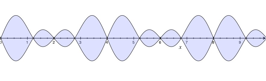 We can make this even more complicated by adding in the following wave:
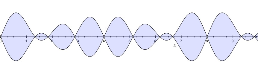 All three displayed algebraic functions share cos(10t), so their common spatial profile reverses sign together. However, sin(πx/4) is nonzero at x=10 m, so the third function also violates a fixed boundary there. For physical fixed-end modes use k_n=nπ/L and ω_n=vk_n instead.
Modes with different frequencies reach their extrema at different times, giving an evolving interference pattern. Such a sum is not automatically a traveling wave; that conclusion requires a particular relationship between its spatial and temporal dependence.
Note:
As a reward for getting to the final section of the final chapter, there will be NO QUIZ! You worked hard to get to the end so it’s the least we can do :)
y₂(x,t)=y₀sin(kx+ωt) (Equation 10.1.2), for the same phase convention as the standing-wave derivation.
L=nλ/2 (Equation 10.1.4), for nonzero normal modes with two fixed ends or two ideal free ends; n=1,2,3,….
T=2π√(L/g) (Equation 10.2.1), for a small-angle simple pendulum.
T=2π√[I/(mgh)] (Equation 10.2.2), for small-angle physical-pendulum motion; I is about the pivot and g is a positive scalar.
Original problem 2
Made the ideal mass–spring model explicit; no source numbers changed.
Problem text
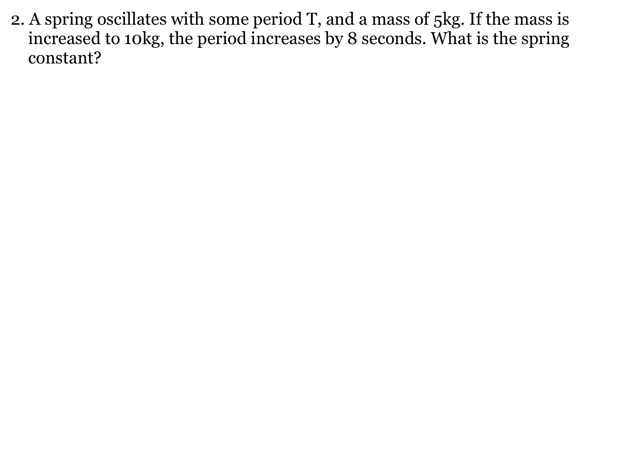
An ideal spring carries a 5 kg mass. Replacing it with a 10 kg mass increases the oscillation period by 8 s. Find the spring constant. Neglect the spring mass and damping.
Drawing is temporarily unavailable. Work on paper if needed, then record your reasoning here.
Saving written working requires JavaScript. The problem remains available above; keep your work on paper or in your own notes.
Original problem 1
Corrected OCR t and stated the endpoint-counting and SI conventions. A standing-wave pattern does not itself travel along the string.
Problem text
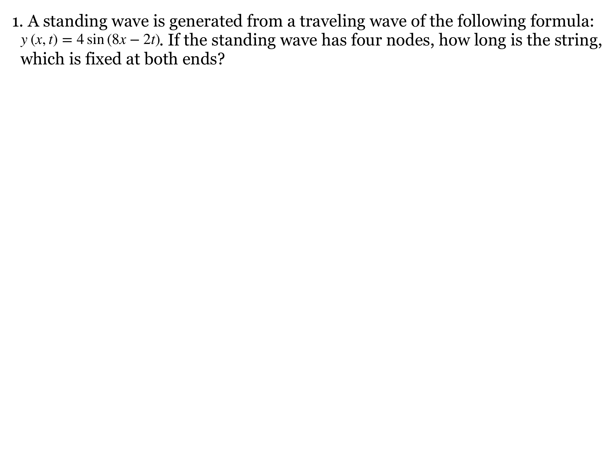
A traveling wave is y(x,t)=4 sin(8x−2t), with x in metres, t in seconds, k=8 rad/m and ω=2 rad/s. It combines with an equal counterpropagating wave to form a standing wave on a string fixed at both ends. If there are four nodes in total, including the endpoints, find the string length.
Drawing is temporarily unavailable. Work on paper if needed, then record your reasoning here.
Saving written working requires JavaScript. The problem remains available above; keep your work on paper or in your own notes.


Original problem 3
The source numbers differ from an exact fundamental by 0.0693%; this is compatible with their displayed precision, but an exact noninteger mode number must not be accepted.
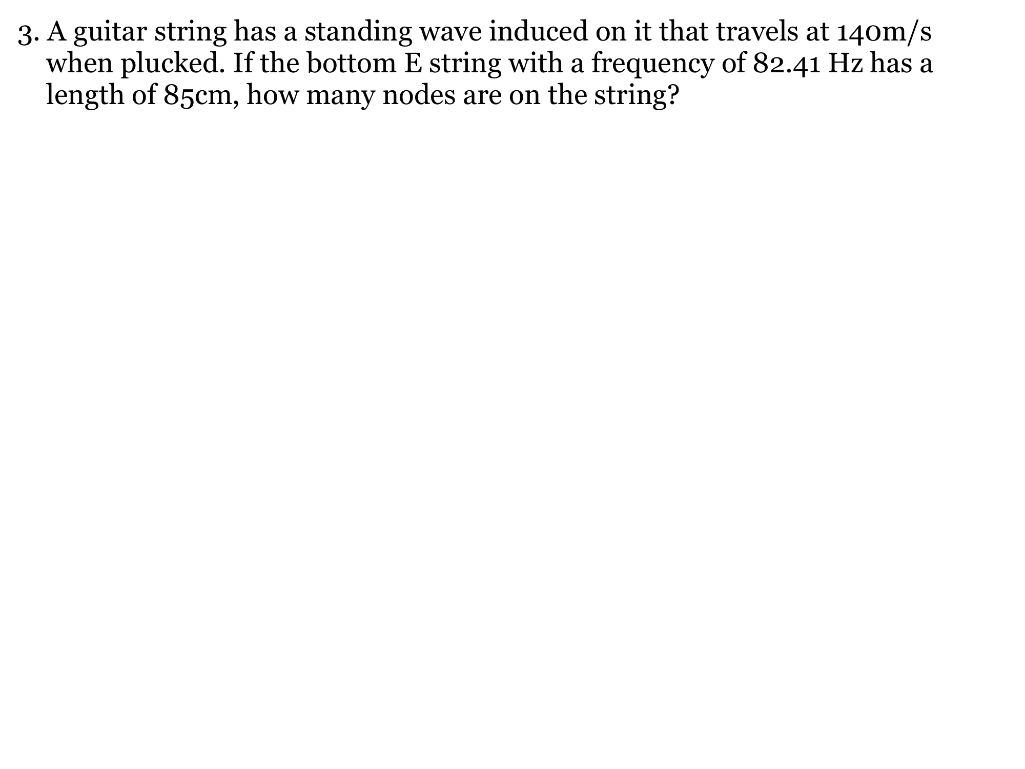
Problem text
The transverse traveling-wave speed on an 85 cm guitar string fixed at both ends is approximately 140 m/s. Its low-E frequency is 82.41 Hz. Determine the intended harmonic and count the nodes, treating the stated speed and length as rounded measurements. Also check whether all three numbers fit an exact normal mode.
Drawing is temporarily unavailable. Work on paper if needed, then record your reasoning here.
Saving written working requires JavaScript. The problem remains available above; keep your work on paper or in your own notes.
Original problem 4
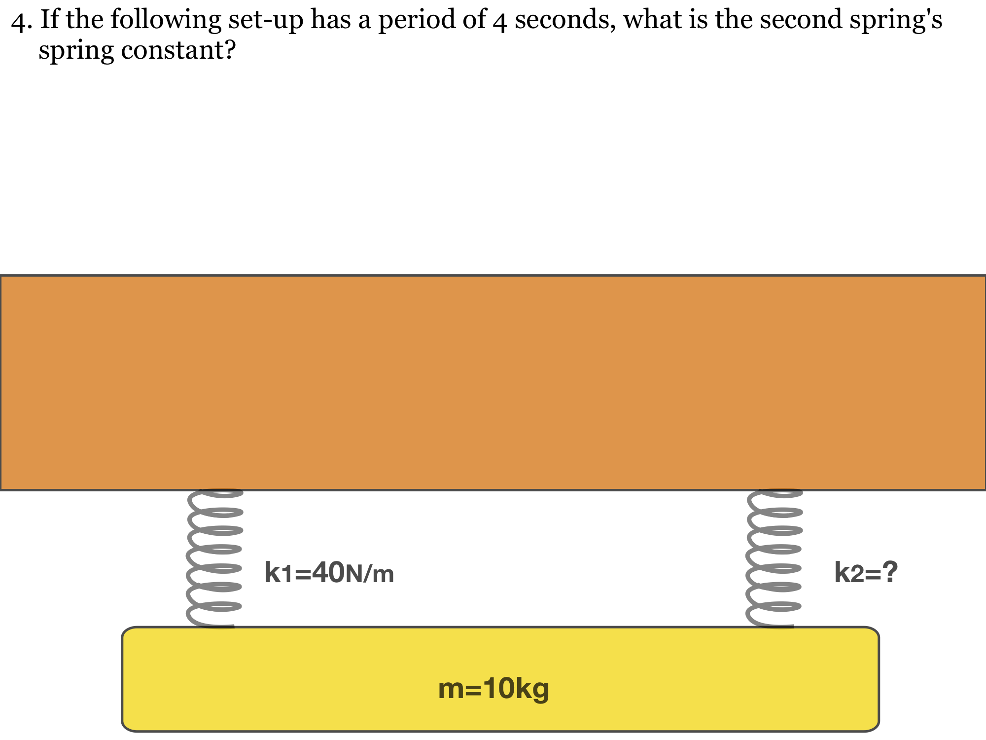
The diagram is parallel, not series. The source period requires negative stiffness; the repaired question retains the data and asks for the consistency check instead of silently changing a number.
Problem text
A 10 kg rigid block hangs from two ideal springs in parallel, as shown in the source diagram. One spring has k₁=40 N/m and the claimed period of pure vertical translation is 4 s. Solve for k₂ and assess whether that value can describe an ordinary positive-stiffness spring.
Drawing is temporarily unavailable. Work on paper if needed, then record your reasoning here.
Saving written working requires JavaScript. The problem remains available above; keep your work on paper or in your own notes.
Original problem 6
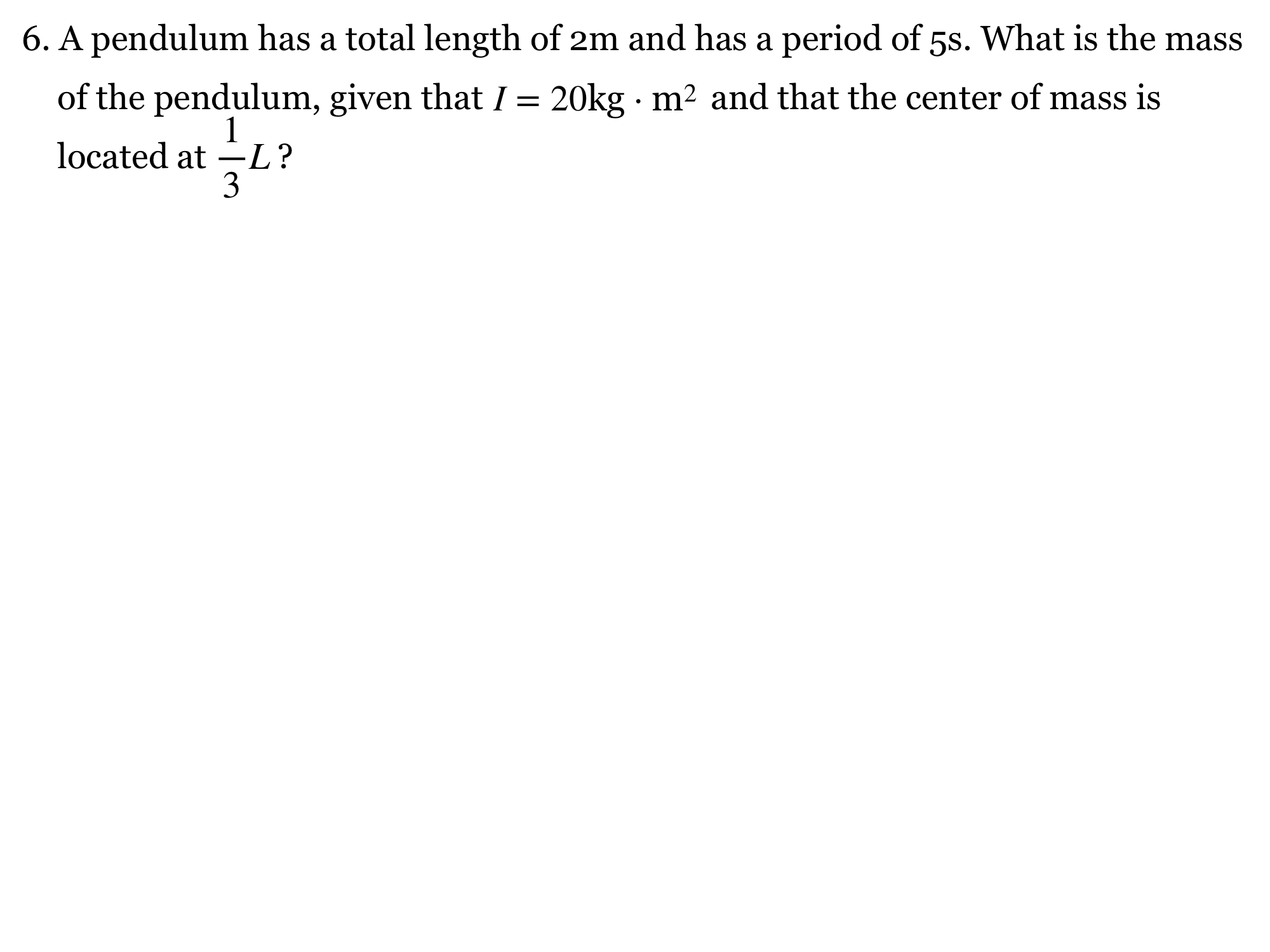
Verified h=L/3 and I=20 kg·m² from the source image. Stated the required pivot-axis inertia and small-angle assumption.
Problem text
A physical pendulum has total stated length L=2 m, pivot-to-centre-of-mass distance h=L/3, moment of inertia about the pivot I=20 kg·m², and small-amplitude period T=5 s. Using g=9.8 m/s², infer its mass from the physical-pendulum period formula.
Drawing is temporarily unavailable. Work on paper if needed, then record your reasoning here.
Saving written working requires JavaScript. The problem remains available above; keep your work on paper or in your own notes.
Original problem 5
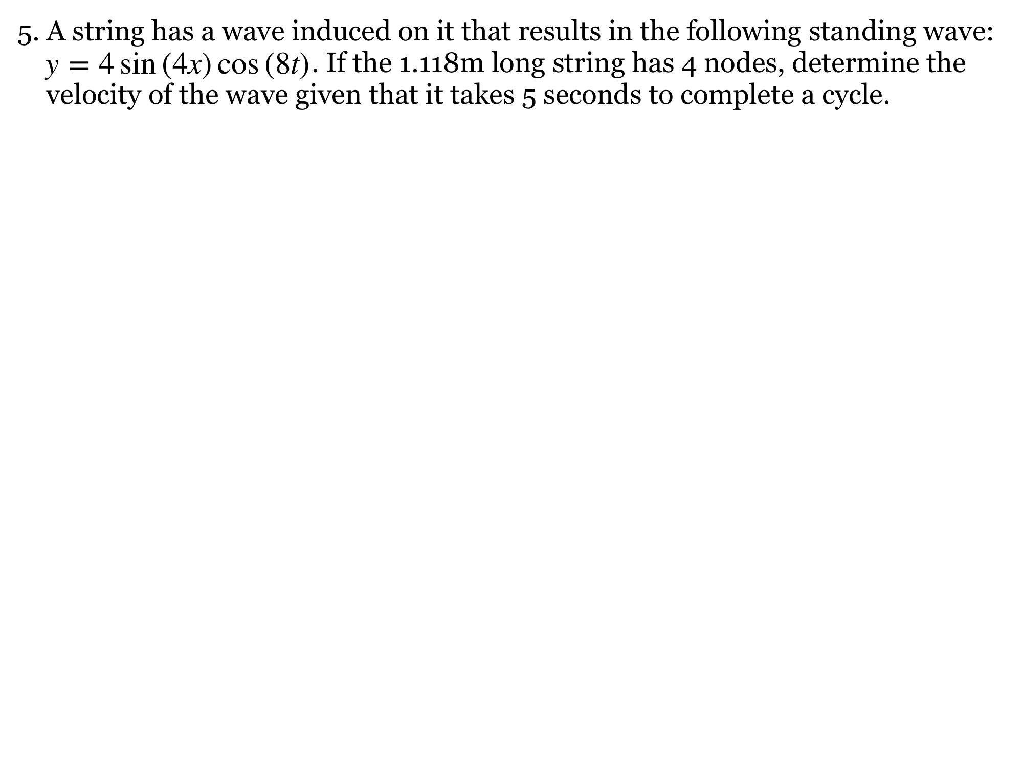
The wave equation, period and stated geometry conflict. Both consistent subsets are evaluated; no missing boundary condition or replacement number is presented as source fact.
Problem text
The source gives y(x,t)=4 sin(4x)cos(8t), a string length of 1.118 m, four nodes, and a period of 5 s. With x in metres and t in seconds, (a) find the component traveling-wave speed from the equation and (b) check the length, node count, and period for mutual consistency. For comparison, find the speed implied solely by L=1.118 m, four total fixed-end nodes and T=5 s.
Drawing is temporarily unavailable. Work on paper if needed, then record your reasoning here.
Saving written working requires JavaScript. The problem remains available above; keep your work on paper or in your own notes.
Original problem 8
Image verification recovers T=10 s. “Loose” alone does not establish a boundary condition. Both endpoint interpretations are explicit; amplitude refers to the standing-wave antinode, not each traveling component.
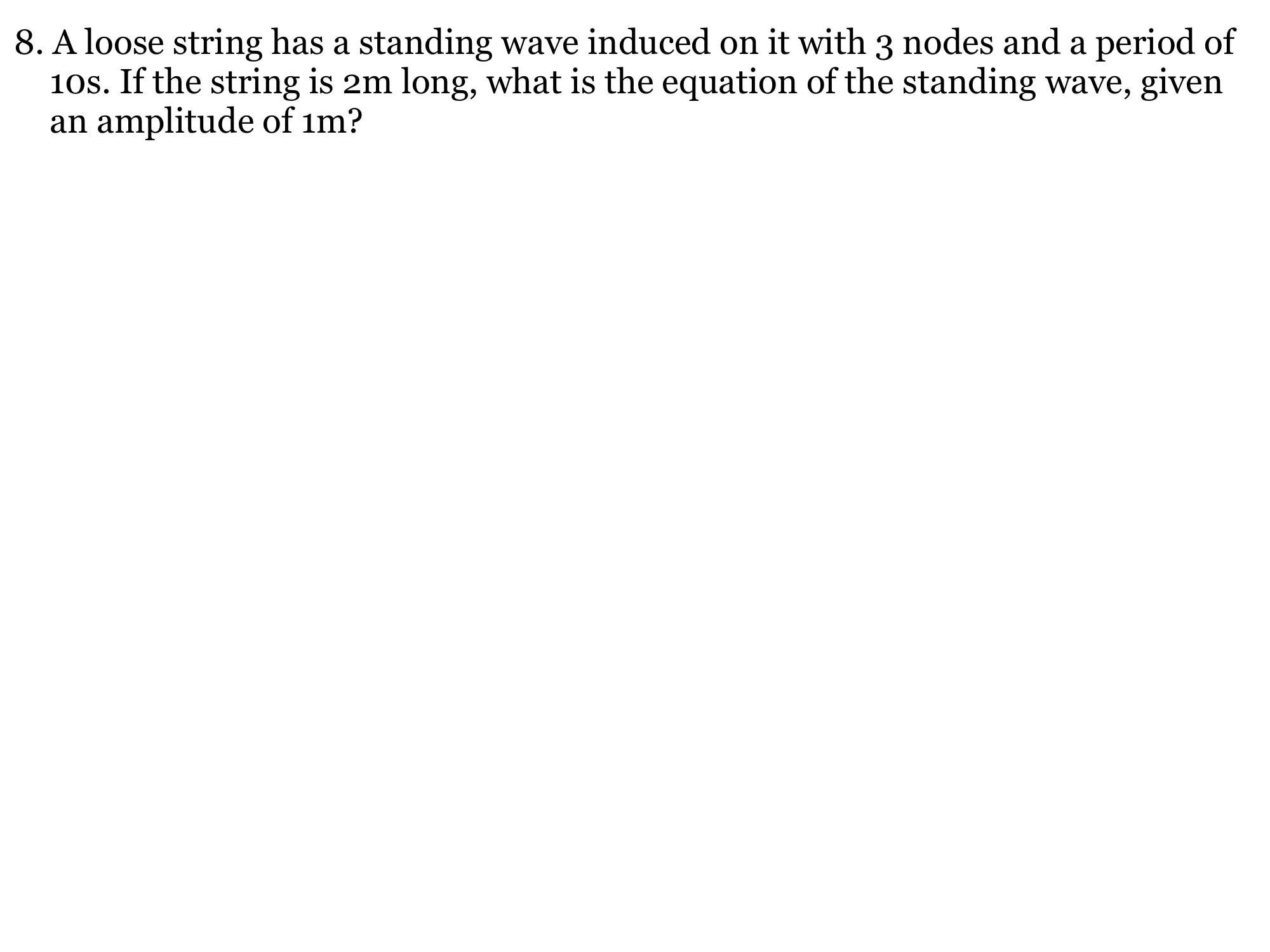
Problem text
A 2 m string has a standing wave with three nodes and period 10 s; its antinode displacement amplitude is 1 m. The source calls it “loose” without specifying its endpoints. Give a valid equation for the intended ideal model with two free ends, placing x=0 at a free end, and explain how the equation changes if both ends are fixed. Choose the time origin at maximum deformation.
Drawing is temporarily unavailable. Work on paper if needed, then record your reasoning here.
Saving written working requires JavaScript. The problem remains available above; keep your work on paper or in your own notes.
Original problem 7
The source does not specify whether 4 m/s belongs to the centre or tip, or whether the sphere is solid/hollow, or a consistent initial phase. The review exposes those limits and gives clearly conditional calculations.
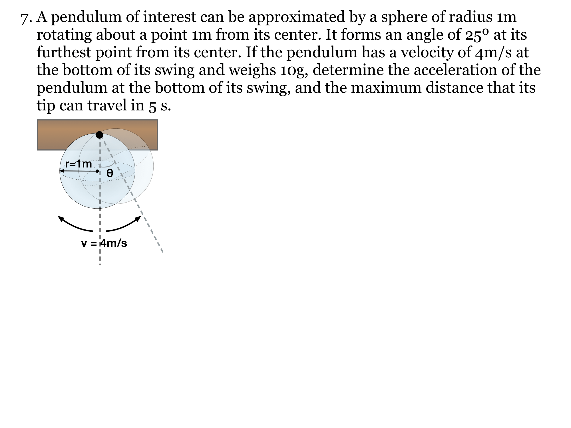
Problem text
A spherical pendulum has radius R=1 m, a pivot 1 m from its centre, mass 10 g, a stated turning angle of 25°, and a stated bottom speed of 4 m/s. The source also asks for the distance traveled by its tip in 5 s. Determine which bottom acceleration can be found, explain the speed-location ambiguity, and check whether the angle and speed can coexist for a uniform solid sphere in conservative motion. Identify what prevents a unique tip-distance answer.
Drawing is temporarily unavailable. Work on paper if needed, then record your reasoning here.
Saving written working requires JavaScript. The problem remains available above; keep your work on paper or in your own notes.
Original problem 10
Restored acceleration units and stated the Earth value used by the chapter.
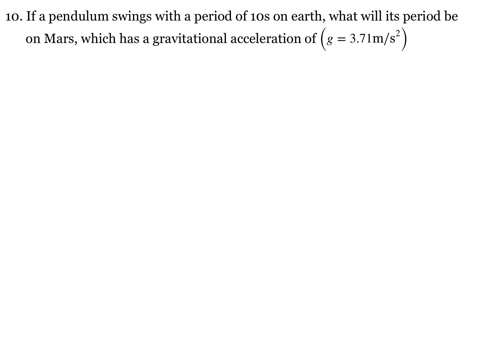
Problem text
The same pendulum has a 10 s period on Earth. Find its period on Mars, where g=3.71 m/s². Take Earth’s g=9.8 m/s² and keep the pendulum geometry and oscillation amplitude unchanged; neglect damping.
Drawing is temporarily unavailable. Work on paper if needed, then record your reasoning here.
Saving written working requires JavaScript. The problem remains available above; keep your work on paper or in your own notes.
Original problem 9
The image exponent is −x/3, not −3x. Replaced x with time because the question describes temporal damping. An exponential envelope does not become exactly zero at a finite time; a detection threshold would be needed for a practical stop time.
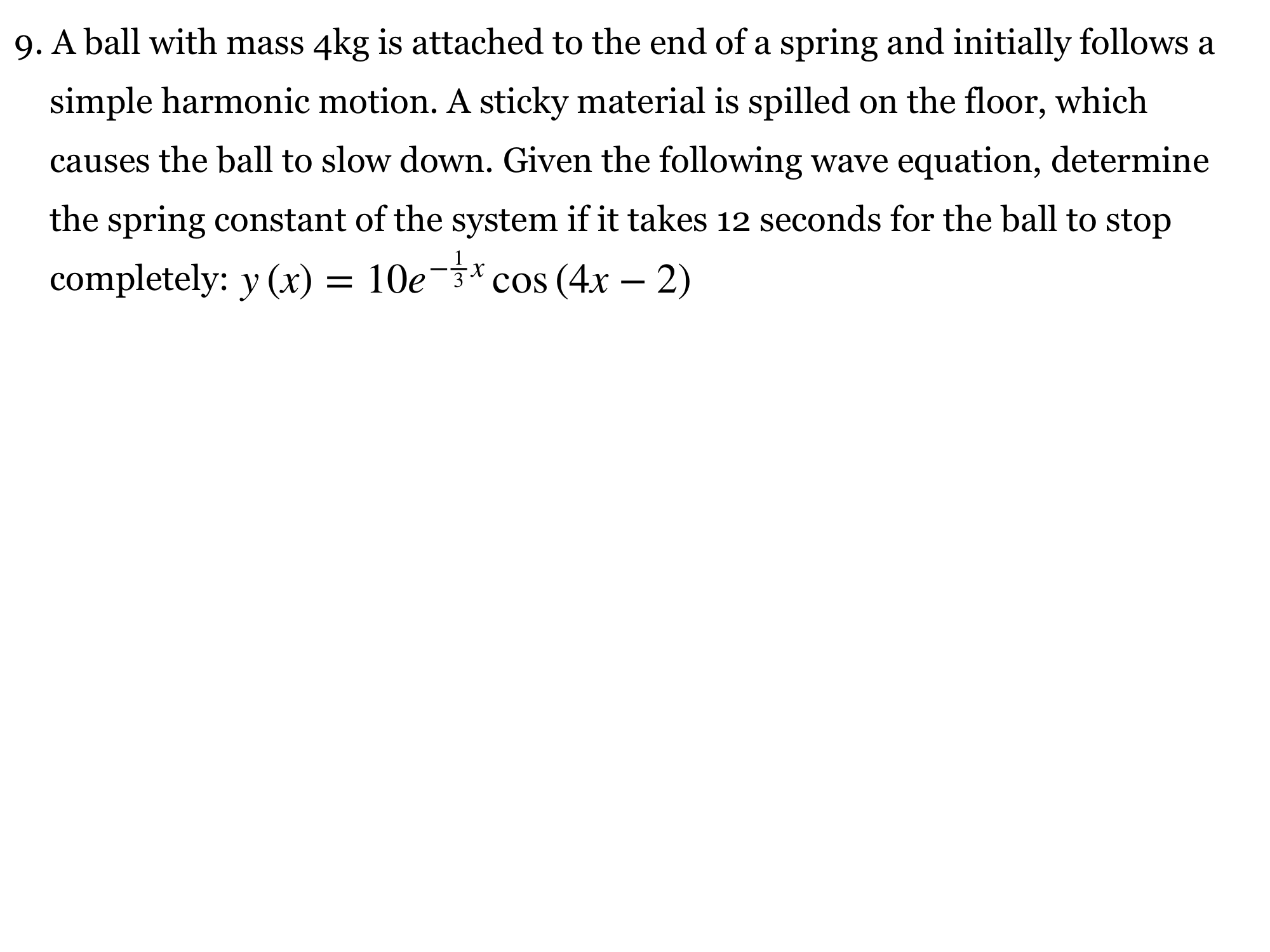
Problem text
A 4 kg mass on a spring follows the damped displacement y(t)=10 exp[−(1/3 s⁻¹)t] cos[(4 rad/s)t−2], where 10 is expressed in the source’s unspecified displacement unit. Assuming linear viscous damping, determine the spring constant. Evaluate the amplitude envelope after 12 s and assess the source’s claim that the mass “stops completely” then.
Drawing is temporarily unavailable. Work on paper if needed, then record your reasoning here.
Saving written working requires JavaScript. The problem remains available above; keep your work on paper or in your own notes.
Want one more challenge?
The original no-quiz finish above is still here. These optional enrichment checks help you test the superposition and boundary-condition ideas. They go beyond this AP Physics 1 course.
Pause & try it
Let's see what stuck.
Choose an answer, then check the reasoning. Try the written problems below before opening their solutions.
0 of 3 checked · 0 correct
Reviewed physics notes (14)
These corrections keep the original lesson’s purpose while fixing errors in the source edition.
- The source’s same-mode sum is still a single mode, while phase matters. — Reference 1
- Correct y(x,y) to y(x,t). — Reference 1
- The combined amplitude is not invariably larger. — Reference 1
- Different k and equal omega do not independently solve one uniform-string wave equation. — Reference 1, Reference 2
- Keep the source figures but state why the advertised free-rope model is not physically admissible. — Reference 1, Reference 2
- The third source profile fails the length boundary, as well as the shared-speed relation. — Reference 1
- Different modal phases alone do not define propagation. — Reference 1
- The source summary had −y₀sin(kx−ωt), which travels in the same direction and cancels y₁ instead of making the displayed standing wave. — Reference 1
- Use scalar g and specify the approximation and inertia axis. — Reference 1
- Replace the spatial variable by time and state the oscillatory regime. — Reference 1
- Use the same damped-frequency notation as the repaired displacement equation. — Reference 1
- The wavelength quantization requires a stated endpoint model. — Reference 1
- Keep the equation-summary approximation explicit. — Reference 1
- State the ideal oscillator model in the summary. — Reference 1
Glossary and deeper reading · 10 refreshers
These editorial refreshers supplement the reading. Definitions and examples are added guidance; original source wording and recorded answers remain in their original context.
-
Simple harmonic motion
Simple harmonic motion occurs when the net restoring force is proportional to displacement from equilibrium and points in the opposite direction. The resulting position varies sinusoidally with time in the ideal model. For example, a mass attached to an ideal spring can execute simple harmonic motion when damping is negligible.
-
Oscillation phase
Phase specifies the position within a repeating oscillation cycle. A phase difference tells how much one oscillation leads or lags another at a chosen place and time. For example, two sinusoidal waves half a cycle out of phase can cancel when their amplitudes are equal.
-
Amplitude
Amplitude is the maximum magnitude of a repeating disturbance measured from its equilibrium value. It describes the size of the oscillation rather than its frequency or propagation speed. For example, pulling a spring-mounted mass farther from equilibrium increases its oscillation amplitude when it is released from rest.
-
Standing wave
A standing wave is a spatially fixed interference pattern formed by suitable waves traveling in opposite directions. Its nodes remain at zero displacement while antinodes mark positions of maximum oscillation amplitude. For example, a string fixed at both ends can support standing waves whose wavelengths fit the boundary conditions.
-
Wave interference
Wave interference is the combination of overlapping wave disturbances. In a linear medium, the signed disturbances add at each location and time without permanently destroying the passing waves. For example, two overlapping upward rope pulses temporarily make a larger upward disturbance.
-
Frequency
Frequency is the number of complete repeating cycles per unit time. It is measured in hertz, meaning cycles per second, and is the reciprocal of the period. For example, a vibrating string with a higher frequency produces more cycles each second.
-
Wave
A wave is a propagating disturbance that can transfer energy without transporting the medium as a whole. Mechanical waves require a material medium, while electromagnetic waves can propagate through vacuum. For example, a pulse travels along a rope while individual rope segments move locally around their equilibrium positions.
-
Superposition
Superposition means adding the separate contributions to obtain a total response in a linear model. Vector fields add vectorially, scalar potentials add algebraically, and wave disturbances add with their signs at each place and time. For example, equal but opposite electric-field contributions can give zero net field at one point while both sources remain present.
-
Pendulum
A pendulum is a system that swings about a support under a restoring torque. A simple pendulum approximates a small mass on a light string and follows simple harmonic motion only for sufficiently small angles. For example, a short string pendulum completes small swings more quickly than a longer one under the same gravitational field.
-
Scalar
A scalar is a quantity described by a value and unit without a spatial direction. A scalar can have a sign when its definition or reference permits one; scalar does not mean always positive. For example, mass is a scalar, whereas the velocity of that mass also needs a direction.