Electric Fields
Construct source-field and net-field representations and explain electrostatic conductor equilibrium.
AP Physics 2 Topic 10.3 · College Board CED printed p. 47, 48 / PDF p. 54, 55 · See this topic in the course outline
The field describes what the source charges do at a place. It lets you predict the force on any small charge you put there.
For another explanation, read The Electric Field. Use the corrected point-source and vector-superposition discussion to practice fields and forces. General quantitative fields within insulators are outside the AP core.
Before you start
- Coulomb’s law and vector components
- Conductor versus insulator
Field belongs to the sources
Charges create electric fields. Define the field at a point with , using a small test charge that does not significantly change the source configuration. The SI unit is N/C, also V/m. “Small” means negligibly perturbing, not a specific charge value. The field exists in the model even when no test charge is there.
A positive source’s field points outward; a negative source’s inward. For a point source in vacuum, . A positive test charge has force along E⃗; a negative test charge has force opposite E⃗ because . Replacing the test charge changes force, not the preexisting source field.
Add arrows, then interpret the map
The net field is the vector sum of the separate source fields: . At each observation point, draw an arrow for each source using the same scale, resolve components, and construct a resultant. Source contributions can cancel in one direction and add in another.
A vector field map places arrows at many locations; direction shows E⃗ and arrow length shows magnitude on a declared scale. A field-line diagram simplifies that map: its local tangent gives direction, and denser lines indicate a stronger field when the drawing uses a consistent line convention. Lines leave positive charge and enter negative charge, and cannot cross at an ordinary point because the net field has one direction there. Field lines are a representation, not rails that constrain a particle’s trajectory.
| Point | Left-source arrow | Right-source arrow | Net result |
|---|---|---|---|
| x = 0 | Right, kQ/a² | Left, kQ/a² | Zero |
| x = 2a | Right, kQ/(9a²) | Right, kQ/a² | Right, 10kQ/(9a²) |
| x = −2a | Left, kQ/a² | Left, kQ/(9a²) | Left, 10kQ/(9a²) |
Use four or fewer source charges for routine calculations. More sources are permitted when high symmetry makes cancellation or addition clear.
Electrostatic equilibrium depends on whether charges can move
In a solid conductor at electrostatic equilibrium, excess charge resides on its surface and the field within the conducting material is zero. Otherwise free carriers would keep accelerating and redistributing, contradicting equilibrium. At its surface, E⃗ is perpendicular: a tangential component would drive surface carriers. This applies to electrostatic equilibrium; a current-carrying resistive wire can have an internal field.
Outside an isolated sphere with a spherically symmetric charge distribution, its field equals that of a point charge of the same net charge at the center. The radius of the sphere matters in deciding whether an observation point is inside or outside. In the metal of a charged solid sphere E = 0, while just outside its surface the field generally is nonzero.
Insulators cannot freely redistribute charge throughout the sample. Excess charge can stay in the interior as well as on the surface, and the internal field may be nonzero in equilibrium. We describe that internal field qualitatively rather than calculating a general insulating charge distribution. A conductor’s zero internal field does not require zero potential: the conductor can sit at one nonzero constant potential.
A cancellation that survives a different test charge
Place +4.0 nC at x = 0 and +1.0 nC at x = 0.30 m. Locate the zero-field point between them, then interpret the force on a negative test charge there.
Let x be the distance from the +4.0 nC source. Between like charges the two field contributions point in opposite directions.
Why this step? A zero field requires opposing vectors; outside this interval they point together.
Set magnitudes equal: . Thus x/(0.30 − x) = 2, so x = 0.20 m.
Why this step? Taking a positive square root is justified because these distances are positive.
The point is closer to the weaker source. E⃗net = 0 gives F⃗ = qE⃗net = 0 for either sign of a sufficiently small test charge.
Why this step? The field is a property of the unchanged sources, rather than of the test charge.
Answer and check
The zero lies at x = 0.20 m. A negative test charge there initially feels zero net electric force; that does not by itself imply stable equilibrium.
A map repeats the same vector operation at many places
A field arrow belongs at an observation point, not at the source that produces it. For every point in a map, first draw the separate source contributions, then add their components. Repeat at multiple locations. Symmetry can make the result zero at one point and large nearby; a zero result at one point does not mean the entire region has zero field.
Declare one arrow-length scale if length represents magnitude. For an isolated point charge, doubling distance makes a field arrow one fourth as long, while its direction remains radial: outward for positive charge and inward for negative charge. A direction-only diagram must say so and cannot be used to compare arrow lengths. The force on a nonperturbing positive test charge follows the field; a negative charge has the opposite force. Its existing velocity still matters to its subsequent path.
Radial arrows with a declared scale
An isolated +2.0 nC point source is at the origin. In vacuum, compare fields at (±0.10 m,0), (0,±0.10 m), (±0.20 m,0), and (0,±0.20 m). Use k = 8.99 × 10⁹ N·m²/C².
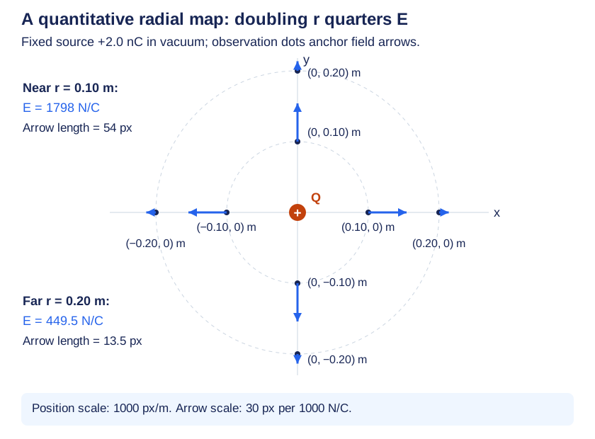
Inspect diagram labels
The diagram keeps its full size here. Focus the view and use the arrow keys, or scroll across it, to inspect every label.
- At radius 0.10 m, E = kQ/r² = 1798 N/C. The four near arrows point right, left, up and down away from the source.
- At radius 0.20 m, E = 449.5 N/C, one fourth the near value. Each far arrow is one fourth as long on the same scale.
- For the figure’s arrow-length scale of 30 pixels per 1000 N/C, near arrows are 53.94 pixels (shown as 54) and far arrows 13.485 pixels (shown as 13.5). The separate coordinate scale is 1000 pixels per meter; arrows start at observation dots.
- Reversing the source reverses all eight arrows without changing their lengths. Reversing a small test charge reverses its force but preserves this source map.
Answer and check
Near fields: 1.80 × 10³ N/C; far fields: 4.50 × 10² N/C. The map uses radial directions and a 4:1 arrow-length ratio.
Make the model respond
Focused Physics 2 model
Two charges: field vectors and potential
Predict first. Can the electric potential be zero while the electric field is nonzero?
E = Σ kq r̂/r² (vector sum); V = Σ kq/r (scalar sum); V(∞) = 0
- E₁
- E₂
- Net E
On a narrow screen, scroll within a figure to read its labels. The table and explanation provide the same physics in text.
Net |E| = 32.36 N/C while V = 0 V. A zero scalar potential does not imply a zero vector field.
Read the model data and comparisons
| Quantity | Value | Unit | Meaning or limit |
|---|---|---|---|
| Point x | 0 | m | |
| Point y | 0.8 | m | |
| Distance r1 | 1 | m | |
| E1,x | 16.18 | N/C | |
| E1,y | 21.57 | N/C | |
| V1 | 26.96 | V | |
| Distance r2 | 1 | m | |
| E2,x | 16.18 | N/C | |
| E2,y | -21.57 | N/C | |
| V2 | -26.96 | V | |
| Net Ex | 32.36 | N/C | |
| Net Ey | 0 | N/C | |
| Net |E| | 32.36 | N/C | |
| Net V | 0 | V |
A positive source produces a field away from itself; a negative source produces a field toward itself. Add x and y components to obtain the vector field. Add signed potentials directly because potential is a scalar. E describes force per positive test charge and V describes potential energy per charge. The displayed arrows are fields, not forces on the source charges.
Assumptions and limits. Stationary point charges in vacuum, at x = ±0.6 m; observation point is in their plane. Potential reference is infinity. Distances at or below 10⁻⁹ m from a nonzero source are excluded. Arrow lengths share one local scale; use the table to compare magnitudes across different control settings.
Try it from memory
Write your answer and reason before opening the worked answer. Your self-assessment is a study decision; it is not an automatically graded score.
Question 1
At a point E⃗ points left with magnitude 400 N/C. What is the force on q = −2.0 μC? Which source-field arrow changes if q doubles?
Worked answer and reason
The force is 8.0 × 10⁻⁴ N right. Doubling q doubles the force magnitude; the source-field arrow remains unchanged if the test charge remains nonperturbing.
A negative charge reverses force direction and the source field does not depend on a small test charge.
Question 2
Compare points inside a charged metal sphere and inside a charged insulating sphere at equilibrium. Can you infer that their potentials are zero?
Worked answer and reason
The field inside the metal is zero; an insulator can have a nonzero internal field. Zero field in the metal implies constant potential, not necessarily zero potential.
Mobility determines charge redistribution; potential depends on the reference choice.
JavaScript enables saved drafts and self-assessment. You can always work on paper.
Catch the tempting mistake
- Electric field points in the direction an electron accelerates.
- Field direction uses positive charge; an electron’s acceleration is opposite.
- Field lines are charged-particle trajectories.
- They show force direction at each place. A particle’s existing velocity can make its path differ.
Put it to work
Give the physical reason as well as the calculation. The worked solutions are on a separate page.
- Problem 5 · vector map
- Problem 6 · radial graph and qualitative comparison
- Problem 15 · experimental potential map and uncertainty
- Problem 17 · source symmetry and energy synthesis
Explain and apply the model
Try these problems before opening the solutions. Show the physical model, your calculation or sketch, and the reason your conclusion follows.
Build a spatial map from two sources
Two fixed +2.0 nC point charges are at (−0.10 m,0) and (+0.10 m,0). Consider M = (0,0), N = (0,0.10 m), S = (0,−0.10 m), and R = (0.20 m,0). Use k = 8.99 × 10⁹ N·m²/C²; sources remain unchanged by any test charge.
(a) Calculate the net field vector at all four points. Construct a labeled spatial vector map with a common arrow-length scale for magnitude. Show the two source contributions at N, explain the cancellations or additions at every point, and mark a zero at M rather than assigning it a direction.
(b) Find the initial electric forces on +1.0 nC and −1.0 nC test charges separately placed at N. Explain why the map is unchanged and whether those forces alone specify each complete future trajectory.
Written working workspace
Drawing is temporarily unavailable. Work on paper if needed, then record your reasoning here.
Saving written working requires JavaScript. Keep your work on paper or in your own notes; the source problem above remains available.
Worked solution and rubric →Revisit the explanation →Revisit the explanation →
Scientific calculator workspace
Keep intermediate precision and report units. This calculator supports arithmetic and elementary functions.
Scientific calculator
This calculator requires JavaScript. Use the physics formula sheets and show your working manually.
+ − * / ^ ! · pi · e · sqrt · sin, cos, tan · asin, acos, atan · atan2(y,x) · ln, log · abs · exp · hypot(x,y). Use * between factors. Keep units in your written working.
For the teacher
- Require separate source-field sketches before net vectors.
- Ask why a tangential surface field contradicts conductor equilibrium.
- Use qualitative reasoning only for fields within general insulators.
Source objectives and scope
- 10.3.A — Describe the electric field produced by a charged object or configuration of point charges.
- 10.3.B — Describe the electric field generated by charged conductors or insulators.
AP Physics 2 only expects students to make calculations of the electric field resulting from four or fewer charged objects or systems. Analysis of the electric field resulting from more charges is allowed in situations of high symmetry. Students will only be expected to perform qualitative analysis of electric fields within insulators.
Suggested skills are teaching guidance. The course applies all science practices across its objectives.
Science references for this teaching
- College Board AP Physics 2 Course and Exam Description, Unit 10 (PDF pages 50–61) — Official topic order, learning objectives, all essential-knowledge clauses, algebra-based scope boundaries; equations visually inspected in local source pages 50,54,56–61.
- OpenStax University Physics Volume 2, 8.5 Molecular Model of a Dielectric — Independent verification that bound polarization leaves a dielectric net neutral and its induced field opposes the free-charge field. All lesson prose and problems are original.
- Corrected original reading: Charge and Matter — Use the corrected charge and Coulomb-law explanations to compare signed charges and pair forces.
- Corrected original reading: Conductors and Insulators — Use the corrected charge-mobility discussion to explain contact, polarization, and grounding with a system boundary.
- Corrected original reading: The Electric Field — Use the corrected point-source and vector-superposition discussion to practice fields and forces. General quantitative fields within insulators are outside the AP core.
- Corrected original reading: The Electric Potential and Potential Energy — Use the corrected algebraic point-charge energy discussion to connect configuration changes with external and electric work.
- Corrected original reading: Calculating Potentials — Use the corrected point-charge scalar sums to practice potential.
- Corrected original reading: Equipotentials, Field lines, and Gradients — Use the corrected contour maps and algebraic field estimates here; calculus-gradient material is an optional extension beyond the AP core.
- Corrected original reading: Capacitors — Use the corrected parallel-plate geometry discussion to compare C, Q, and voltage.
- Corrected original reading: Stored Energy and Dielectrics — Use the corrected energy and dielectric discussion with an explicit fixed-Q or fixed-voltage constraint.
Glossary and deeper reading · 13 refreshers
These editorial refreshers supplement the reading. Definitions and examples are added guidance; original source wording and recorded answers remain in their original context.
-
Electric charge
Electric charge is a conserved property that determines electric interactions. It can be positive or negative and is measured in coulombs; ordinary net charges arise from an imbalance of charged particles. For example, transferring electrons between initially neutral objects leaves one negatively charged and the other positively charged.
-
Vector
A vector is a quantity with a magnitude and a direction, represented by an arrow or by components along chosen axes. Vectors add by adding corresponding components rather than simply adding their magnitudes. For example, an eastward displacement followed by a northward displacement produces a resultant pointing northeast. The zero vector has zero magnitude and no unique direction.
-
Superposition
Superposition means adding the separate contributions to obtain a total response in a linear model. Vector fields add vectorially, scalar potentials add algebraically, and wave disturbances add with their signs at each place and time. For example, equal but opposite electric-field contributions can give zero net field at one point while both sources remain present.
-
Coulomb’s law
Coulomb’s law gives the electric force between point charges using their charges and separation. The magnitude grows with the product of the charge magnitudes and decreases with separation squared, with the medium accounted for in the stated model. For example, doubling the separation of two fixed point charges reduces the force magnitude to one quarter.
-
Vector component
A vector component describes the part of a vector along a chosen axis. Its signed value changes when the axes change, even though the physical vector remains the same. For example, a diagonal launch velocity can be resolved into horizontal and vertical components that share the same elapsed time.
-
Magnitude
Magnitude is the nonnegative size of a vector quantity. It does not specify direction, and it differs from a signed component. For example, a westward velocity can have a negative x component while its speed, the velocity magnitude, stays positive.
-
Field line
A field line is a drawn curve whose tangent shows the local direction of a vector field. Closer spacing conventionally represents greater field strength, and lines are a representation rather than physical threads. For example, electric field lines point away from a positive point charge and toward a negative one.
-
Electrical conductor
An electrical conductor contains charge carriers that can move through the material. In electrostatic equilibrium, mobile charges redistribute until the electric field within the conducting material is zero. For example, excess charge on an isolated metal object resides on its surface after the charges settle.
-
Electrostatic equilibrium
Electrostatic equilibrium is a condition in which the charge distribution has settled and there is no sustained motion of free charges. Within the material of an ideal conductor, the electric field is zero and the connected conductor is at one potential. For example, charges on a metal surface rearrange until any tangential surface field that would drive them has vanished.
-
Electrical insulator
An electrical insulator strongly restricts the movement of charge carriers through its bulk. Its bound charges can still rearrange slightly to polarize in an applied electric field. For example, a plastic rod can retain localized excess charge even though it does not conduct current like a metal wire.
-
Velocity
Velocity describes how position changes with time and includes direction. Instantaneous velocity describes one moment, while average velocity is displacement divided by elapsed time. For example, a car turning a corner can change velocity while maintaining the same speed.
-
Electric force
Electric force is the interaction of an electric field with a charged object. For point charges at rest, like signs repel and opposite signs attract, with direction along their separation. For example, an electron and proton exert equal-magnitude opposite forces on one another despite having different masses.
-
Force
A force describes an interaction that can change an object’s momentum. It is a vector measured in newtons, so both size and direction matter when forces are added. For example, a rope can pull a cart while the floor exerts friction in another direction.