Equipotentials, Field lines, and Gradients
Beyond AP Physics 1
Original source retained for reference; this draft does not establish AP coverage.
Original author draft. Original wording and recorded answer states are preserved without claiming reviewed scientific correctness or AP alignment.
Physics 2 original textbook · Chapter 2
Section 3 Overview
Section 3
Equipotentials, Field lines, and Gradients
In chapter 1 section 2 we briefly discussed electric field lines and their relation to charges. Here we introduce a new concept, the equipotential. Equipotentials show us where the potential is the same value. Around lone point charges equipotentials manifest as circles. This is because the potential will depend only on the distance from a single charge. That distance forms the radius of the equipotential circle.
Very near an isolated point charge, its potential dominates other finite contributions. Far from a localized distribution with nonzero total charge Q, the leading potential is and equipotentials approach spheres (circles in a plane). For a neutral distribution, the monopole term vanishes; a dipole’s angular dependence remains, so the point-charge far-field claim does not apply.
Example 2.3.1
Find equipotential voltages at radii 1 m, 2 m, and 4 m from a +1 nC point charge.
Authored clarification: V(∞)=0; surfaces are spheres and planar cross sections are circles.
Since we are dealing with a point charge the equipotentials will be circular. To calculate the voltage at these equipotentials all that’s necessary is to calculate the voltage at that radii given.
For the equipotential at 1m we have that

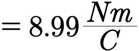
For equipotential at 2m we go through a similar calculation

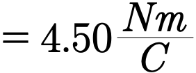
Finally for the equipotential at 4m we have that

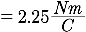
Gallery 1.1 Equipotentials
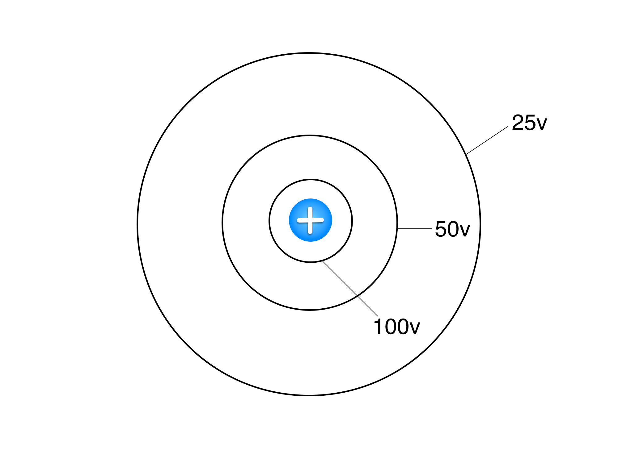
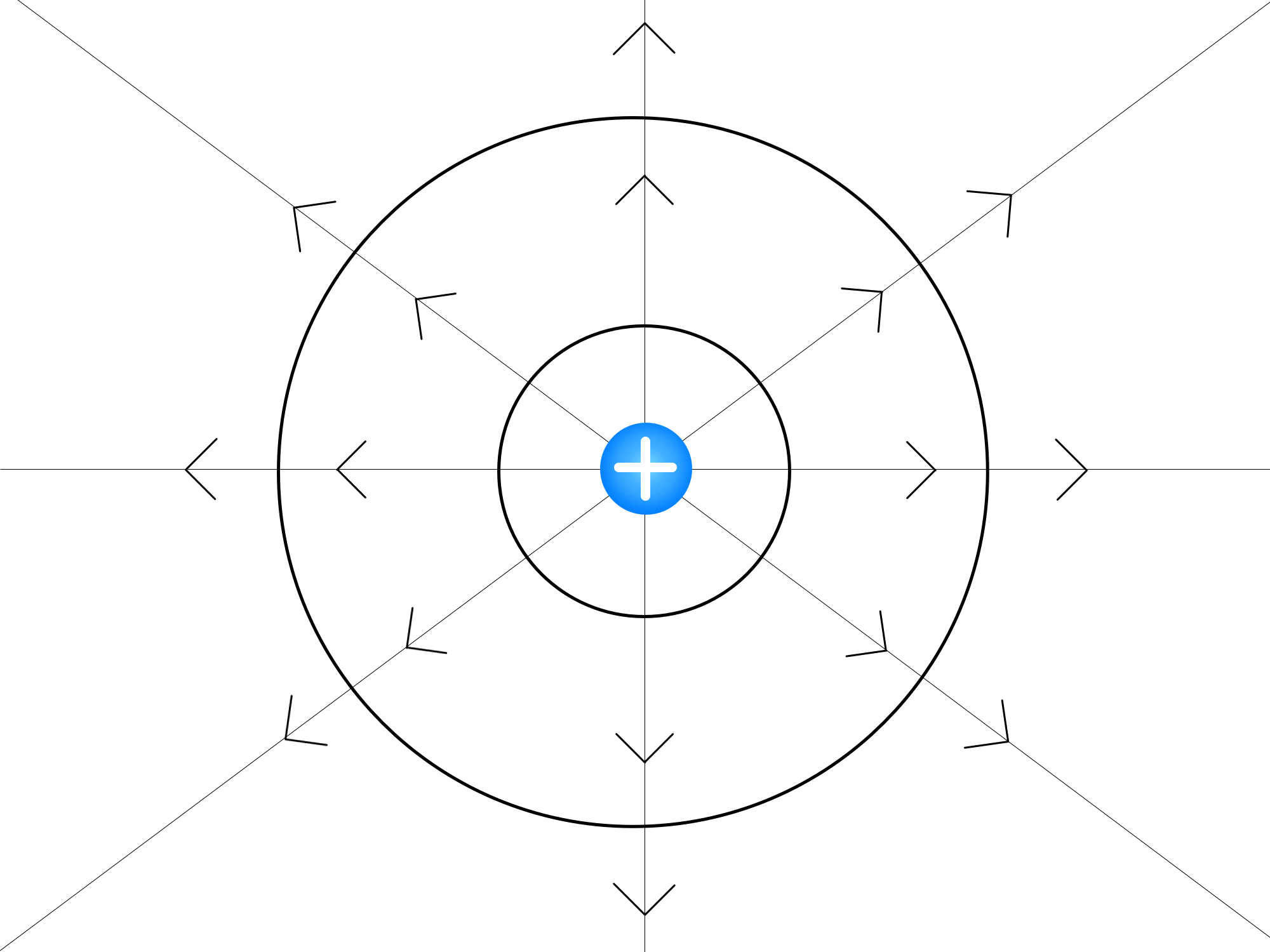
The radial dependence of the electric potential causes a point charge to carry circular equipotentials (lines of constant potential). For a positive charge it follows that at a equipotential the value of the electric potential will be a positive value.
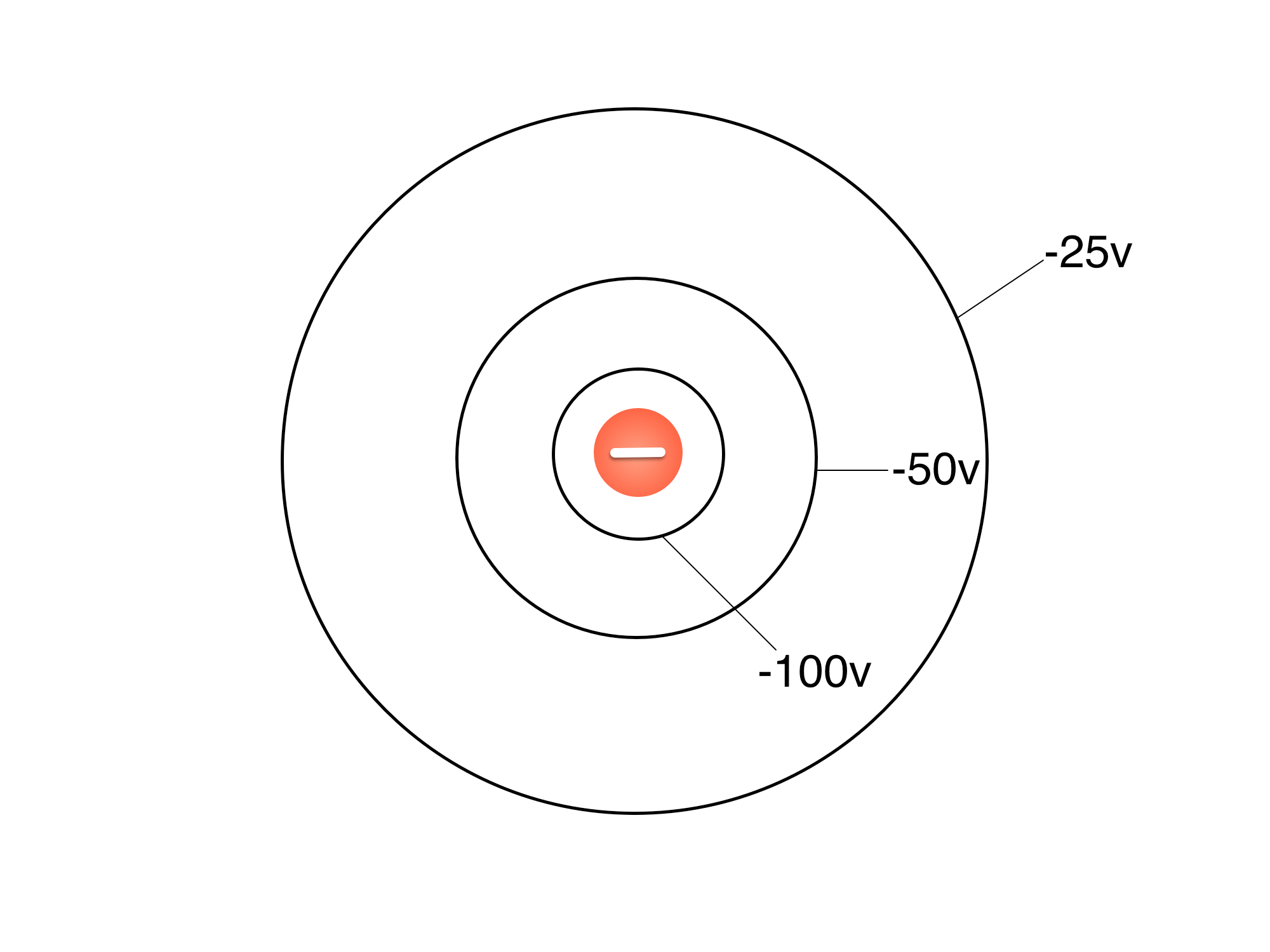
For a negative point charge we also have circular equipotentials. Unlike the positive charge the equipotentials instead hold negative values.
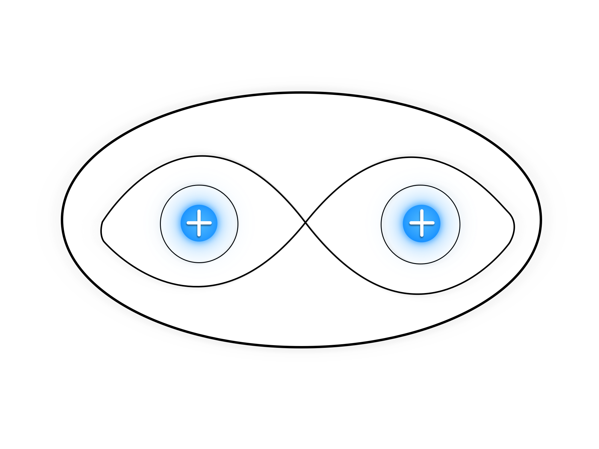
When more than single point charge (or charge distribution) is placed into some configuration the equipotential takes on progressively more interesting shapes. As you can see here the equipotential crosses itself when close to the charges but as you get further out the equipotential begins to resemble that of a point charge.
A curious fact about the equipotential and field lines is that when they are plotted alongside one another they are always perpendicular whenever they cross. Even more interesting is that electric field lines always point in the direction of decreasing electric potential. This relationship is not just a simple coincidence.
Mathematically this relationship can be expressed as negative the gradient of the electric potential. The gradient is one way to represent the slope of a multivariable function. We define it as follows.
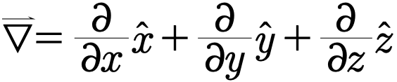
Where the symbols
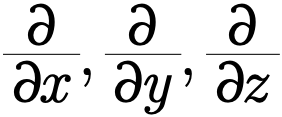
are partial derivatives which are evaluated by taking the derivative of something with respect to the given variable while holding all other variables constant.
Interactive 1.6 Field Lines and Equipotentials
Decreasing Direction
Refer to the first gallery image of this section. As you get further from the charge you will see the value of the equipotentials decrease. The field line then points in the direction of decreasing potential.
Perpendicularity
Notice how every field line is perpendicular to the equipotentials is crosses.
Example 2.3.2
Take gradients of f=xyz and g=ln(x²y²z²).
Authored clarification: This is a calculus extension; g is defined where x, y and z are nonzero.
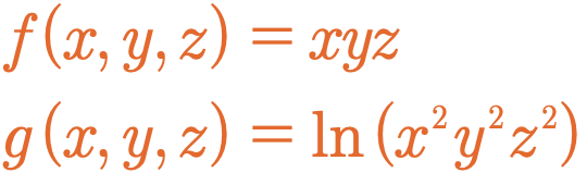
This is brief exercise to get comfortable with gradients. If we look at the first function f and apply the gradient operator and go no further we get that

Let’s look at an individual differential.
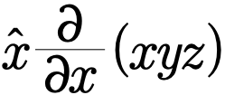
Taking the partial derivative with respect to x means that we must pretend that every variable besides x is a constant then take the derivative with respect to x. This gives us that
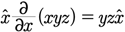
Since x was not composed with any other function and was raised to only the first power it becomes a 1. Since everything else was treated as a constant it stays untouched as would expect for a constant multiple.
|In this particular example the same occurs for all other terms. For the gradient of f we then have
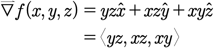
We now turn to g. Writing out the gradient applied to g we have that

Taking a look at the first term again we have
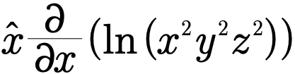
Notice that to differentiate this we must use the chain rule. Differentiating the outside function and then the inside function as we would with a normal derivative. Remember that since we are taking the partial derivative with respect to x we must treat all other variables as constant. Doing so gives us

Since the y and z components are of the same form their partials are similar. After computing them we finally get that

Example 2.3.3
Optional gradient method for a point-charge field. Prerequisites: partial derivatives of a multivariable potential; the physical point-charge field can also be used directly. This preserved source example makes no AP coverage claim.
Use V=kQ/√(x²+y²) to find E for a point charge at the origin in the xy plane.
Authored clarification: V(∞)=0; the origin is excluded.
This example will be a little technical so bear with me. Here we are showing that negative the gradient of the electric potential of a point charge does indeed give us the electric field of that point charge. The first thing we will want to do is go ahead and expand both the gradient operator and r.
The gradient operator has been defined for us and r is nothing more than the length of a line in our chosen coordinate system. We will use 2-d coordinates. This means that we have

From here we will focus only on single term of the above expression to make everything clear
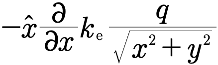
Partials carry many of the same properties of a normal derivative. Being able to pull out constants is one of them so that the above becomes
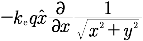
The next part now requires us to understand that a partial is only slightly different from the derivatives in that we only treat
x as a variable and pretend y is constant. Since the chain rule holds for partial derivatives this means that

where
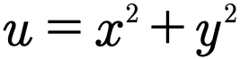
Doing the above derivatives finally gives us that

The same process is repeated for y so that

If we put the above solutions together we get

or slightly more compactly

If we wish we can easily simplify this by substituting in r. Doing so gives us the following
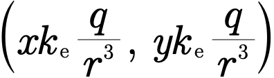
Factoring the equation then gives us
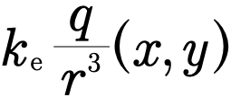
Which through recognizing that the vector is nothing more than the radial vector we can transform the above into the electric field of a point charge.

Review 1.3 Section 3 Review
This review preserves the author’s recorded prompts, choices, and answer states. Corrected items have separate reviewed explanations and keys; unchanged draft keys are marked unreviewed. Unfinished items are not scored.
Original question 1
Where E is nonzero in electrostatics, how does E meet a smooth equipotential surface?
Perpendicularly
Tangentially
At any angle
Reviewed answer and reasoning
A
E=−∇V is normal to a surface of constant V. At a zero-field point its direction is undefined.
This reviewed version states the assumptions or convention needed for one determinate answer. The archived source prompt and key are retained.
Archived original question and recorded key · contains the source error
Electric Field lines are always perpendicular to equipotentials.
True
False
Original recorded key: A
Original question 2
Field lines point in the direction of increasing potential
True
False
Reviewed answer and reasoning
B
E points toward decreasing potential, so false.
The independent semantic audit confirms this source prompt and recorded key under its stated conditions.
Archived original question and recorded key · contains the source error
Field lines point in the direction of increasing potential
True
False
Original recorded key: B
Original question 3
Two equal-magnitude point charges +Q and −Q are equidistant from a midpoint. With V(∞)=0, what is V there?
0
Cannot be zero for opposite charges
Reviewed answer and reasoning
A
Potential is a scalar: . Equal distances and equal magnitudes are essential.
Authored correction or explicit assumptions; this reviewed key is separate from the archived original recorded states.
Archived original question and recorded key · contains the source error
Two oppositely charged particles are placed near one another. What is the value of the equipotential halfway between them?
-20 V
-10 V
10 V
20 V
None of the above
Original recorded key: A
Original question 4
The electric field and electric potential are related through the gradient operator.
True
False
Reviewed answer and reasoning
A
E=-gradient V for electrostatics.
The independent semantic audit confirms this source prompt and recorded key under its stated conditions.
Archived original question and recorded key · contains the source error
The electric field and electric potential are related through the gradient operator.
True
False
Original recorded key: A
Original question 5
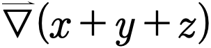
Calculate
0
3
None of the above
Reviewed answer and reasoning
D
Gradient of x+y+z is xhat+yhat+zhat, not scalar 3.
The independent semantic audit confirms this source prompt and recorded key under its stated conditions.
Archived original question and recorded key · contains the source error
Calculate
0
3
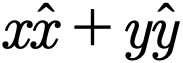
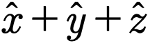
None of the above
Original recorded key: D
Chapter 2 Problems
Four point charges each equal to −Q, Q>0, are at (±a,±a), with a=1 m. Find the potential at the origin using V(∞)=0.
Authored clarification: The original says “negative charges of charge q”; Q here is the positive magnitude, so each source is −Q.
Optional original-source extension. Prerequisites: ideal infinite-sheet fields, signed potential differences and energy conservation. This item makes no AP coverage claim.
Infinite sheets at x=0 and x=d>0 have surface densities +σ and +2σ. Find V(d)−V(0) and the energy change for a test charge q moved from 0 to d. Which charge sign could accelerate from rest in that direction?
Authored clarification: σ>0 denotes surface density, not a finite total charge. The motion starts at the +σ sheet and ends at the +2σ sheet.
Optional original-source extension. Prerequisites: scalar potential superposition for ideal thin rings and a reference at infinity. This item makes no AP coverage claim.
Two thin uniformly charged rings of radius R share a center and lie in perpendicular planes. Their total charges are Q₁ and Q₂. Find the potential at the common center with V(∞)=0.
Authored clarification: The original does not give the ring charges; Q₁ and Q₂ are explicit independent parameters.
Optional original-source extension. Prerequisites: continuous surface charge, a definite integral and electric potential energy. This item makes no AP coverage claim.
A thin disk of radius R and uniform total charge Q lies in the xy plane. Find V(h) on its axis for h≥0 with V(∞)=0, and ΔU for a test charge qₜ moved quasistatically from the center just above the disk to height h.
Authored clarification: The disk charge Q and moving test charge qₜ are distinct. The initial location and potential reference are now specified.
Optional original-source extension. Prerequisites: an ideal infinite-line field, a radial potential integral and logarithms. This item makes no AP coverage claim.
An infinitely long wire has uniform line charge density λ. Determine V(d) with the finite reference V(r₀)=0.
Authored clarification: The reference radius r₀>0 and line density λ are essential; an ideal infinite line does not admit V(∞)=0.
Define an equipotential and describe the equipotential surfaces of an isolated point charge Q using V(∞)=0.
Authored clarification: Treat Q as a nonzero isolated point charge in three dimensions. Describe the full surfaces and a cross section in a plane through the charge.
Explain the relation between equipotentials and electric field lines. For a negative point charge −Q, Q>0, does potential increase or decrease as radius increases?
Authored clarification: The source sentence ends unfinished. This explicitly completes the comparison using increasing radius and V(∞)=0.
Optional original-source extension. Prerequisites: partial derivatives and the potential-gradient relation. This item makes no AP coverage claim.
A potential is . Find the electric field.
Authored clarification: This transcribes the original formula image with coefficients a and b to make its units explicit; the source image corresponds to a=b=1 in its chosen units.
Reviewed worked examples
These authored derivations are paired with the original example identities. Added assumptions are stated.
Example 2.3.1 · reviewed solution
Find equipotential voltages at radii 1 m, 2 m, and 4 m from a +1 nC point charge.
Authored clarification: V(∞)=0; surfaces are spheres and planar cross sections are circles.
Use point-charge potential.
Substitute kQ≈8.98755 V·m.
Evaluate radius 4 m.
The voltages are approximately 8.99 V, 4.49 V, and 2.25 V.
Check
Doubling radius halves potential.
Example 2.3.2 · reviewed solution
Take gradients of f=xyz and g=ln(x²y²z²).
Authored clarification: This is a calculus extension; g is defined where x, y and z are nonzero.
Differentiate f while holding the other coordinates fixed.
Use the chain rule on g.
Repeat cyclically.
Check
The log argument requires xyz≠0; absolute-value log equivalents give the same derivatives.
Optional gradient method for a point-charge field. Prerequisites: partial derivatives of a multivariable potential; the physical point-charge field can also be used directly. This preserved source example makes no AP coverage claim.
Example 2.3.3 · reviewed solution
Use V=kQ/√(x²+y²) to find E for a point charge at the origin in the xy plane.
Authored clarification: V(∞)=0; the origin is excluded.
Electric field is the negative gradient.
Differentiate the potential.
Apply both minus signs.
Check
For positive Q, E points outward; a positive expanded gradient would give the wrong sign.
Glossary and deeper reading · 4 refreshers
These editorial refreshers supplement the reading. Definitions and examples are added guidance; original source wording and recorded answers remain in their original context.
-
Equipotential
An equipotential is a set of locations with the same electric potential. Moving a charge along it produces no electric potential-energy change, and electric field vectors are perpendicular to its surface. For example, concentric spherical surfaces around an isolated point charge are equipotentials.
-
Field line
A field line is a drawn curve whose tangent shows the local direction of a vector field. Closer spacing conventionally represents greater field strength, and lines are a representation rather than physical threads. For example, electric field lines point away from a positive point charge and toward a negative one.
-
Electric field
An electric field assigns the electric force per unit positive test charge to each location. The field is produced by the sources and is a vector, while the force on a negative charge points opposite the field. For example, the electric field between ideal parallel capacitor plates can accelerate an electron opposite the field arrows.
-
Electric charge
Electric charge is a conserved property that determines electric interactions. It can be positive or negative and is measured in coulombs; ordinary net charges arise from an imbalance of charged particles. For example, transferring electrons between initially neutral objects leaves one negatively charged and the other positively charged.