Displacement, Velocity, and Acceleration

Time fits into the picture

We’ve discussed where an object starts and finishes. What we haven’t included yet is how long the trip takes. A cart covering 8 m in 2 s behaves differently from one covering those same 8 m in 20 s, even though their displacements match.

For translational motion, the object model treats the cart as one point, ignoring size, shape, and internal configuration. Mass stays part of the model. This is useful when wheel rotation and deformation don’t matter to the question. The point must be tracked consistently; switching between the front and back of the cart creates fake displacement.

Displacement is Δx = x_f − x_i. Elapsed time is Δt = t_f − t_i. Average velocity describes the entire interval: v_avg = Δx/Δt. Its unit is m/s. Average speed instead uses total distance divided by elapsed time. A round trip can therefore have zero average velocity and a nonzero average speed.

View diagram at full size ↗

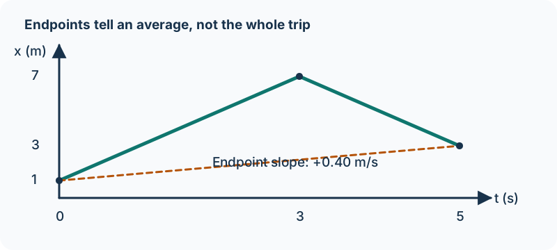
Example 1.2.1 — A cart that changes its mind

A cart starts at x = 1 m at t = 0 s, reaches x = 7 m at t = 3 s, and returns to x = 3 m at t = 5 s. Its total displacement is 3 − 1 = +2 m. Its average velocity over the whole trip is +2/5 = +0.40 m/s. The distance is 6 + 4 = 10 m, giving an average speed of 2.0 m/s.

Neither average says that the cart moved at that value at every instant. The endpoints discard the information about the reversal. That’s why the same average velocity can describe many different trips. A position–time record provides more information than just the first and final entries.

Acceleration is about a change in velocity, not position alone. a_avg = (v_f − v_i)/Δt, with units m/s². Suppose a different cart changes from +6 m/s to +2 m/s in 2 s. Its average acceleration is (2 − 6)/2 = −2 m/s². It moves right but slows down. If it changes from −2 m/s to −6 m/s in 2 s, the acceleration is also −2 m/s², but now it speeds up while moving left.

Smaller intervals show the moment

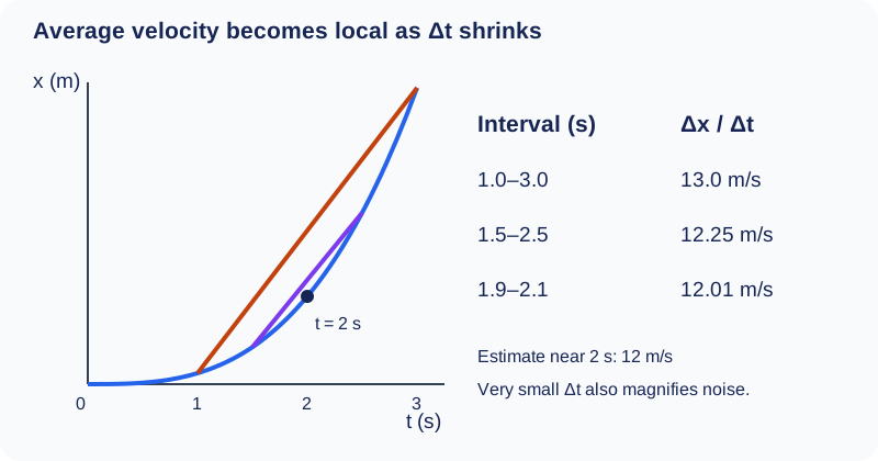
An instantaneous velocity describes motion at a particular moment. Estimate it by measuring displacement over a short time interval centered near that moment. As the interval gets shorter, the average better approximates the instantaneous value, provided measurement uncertainty is controlled. Instantaneous acceleration can likewise be estimated from velocity changes over short intervals. No calculus calculation is required here.

A curved path adds another way to accelerate: the velocity’s direction can change while its magnitude stays fixed. A car rounding a bend at constant speed is accelerating. In one dimension, a sign change in velocity also indicates a direction change, but it takes place through intermediate velocities rather than an actual instantaneous jump for a finite force.

Read signs together

The sign of position tells you which side of the origin you’re on. The sign of velocity tells you which way you’re moving. The sign of acceleration tells you how velocity changes. Those three signs need not match. A cart at a positive position can move left and slow down, so x is positive, v is negative, and a is positive.

Try filming a cart beside a meter ruler with a fixed camera. Record position at equally spaced times. Compute average velocities between neighboring frames, then compare values from longer and shorter time intervals. Use a visible scale in the same plane as the cart to reduce perspective error. Very short intervals magnify position-reading uncertainty: if the displacement is barely larger than the uncertainty, more frames aren’t automatically better. A useful experimental argument names both the improved time resolution and that tradeoff.

Example 1.2.2 — A model choice and a shrinking interval

A 0.50 kg charged cart travels across a 10 m track. To predict only its translational position, represent it by a single tracked point and retain its mass and total charge. The object model ignores the cart’s size, shape, and internal configuration. It cannot tell us how its wheels turn or how the chassis bends; those questions require the discarded structure. Charge is an example of an extensive property carried by the model, although quantitative electric-force analysis is outside AP Physics 1.

In a separate motion trial on a longer track, suppose a smooth position record gives x = 1.000, 3.375, 6.859, 8.000, 9.261, 15.625, and 27.000 m at t = 1.0, 1.5, 1.9, 2.0, 2.1, 2.5, and 3.0 s. Around t = 2.0 s, the average velocities over 1.0–3.0 s, 1.5–2.5 s, and 1.9–2.1 s are 26/2 = 13.0 m/s, 12.250/1 = 12.25 m/s, and 2.402/0.2 = 12.01 m/s. The successively shorter secants suggest an instantaneous velocity near 12 m/s at 2.0 s. We estimated a local value from measurements; we did not assume uniform acceleration or solve a variable-acceleration equation.

For a separate smooth velocity record with the same numerical values in m/s at those times, the average accelerations around 2.0 s are 13.0, 12.25, and 12.01 m/s². The small-interval estimate approaches an instantaneous acceleration near 12 m/s². These are different physical records: the first divides position change by time; the second divides velocity change by time. A smaller interval improves locality, but noise divided by a very small elapsed time can worsen the uncertainty.

Inspect diagram labels

The diagram keeps its full size here. Focus the view and use the arrow keys, or scroll across it, to inspect every label.

View diagram in a separate tab ↗

Check what you know

Pause & try it

Let's see what stuck.

Choose an answer, then check the reasoning. Try the written problems below before opening their solutions.

0 of 3 checked · 0 correct

1. A runner returns to the start after 20 s. Which statement must be true?

Average velocity is zero Average speed is zero Instantaneous velocity was always zero

Check my answer

Read the worked solution →

2. Velocity changes from −3 m/s to −7 m/s in 2 s. What is the average acceleration?

+2 m/s² −2 m/s² −5 m/s²

Check my answer

Read the worked solution →

3. A car travels around a circular bend at fixed speed. Is it accelerating?

No; only changing speed causes acceleration Yes; the velocity direction changes Only if its position is negative

Check my answer

Read the worked solution →

Give it a try

Practice 1

A tracker gives positions 0 m, 2 m, and 8 m at times 0 s, 1 s, and 3 s. Calculate average velocity during each interval and during the full 3 s.

Full worked solution

Practice 2

A cart moving right has positive acceleration. Describe what happens to its speed. Then repeat for a cart moving left with the same positive acceleration.

Full worked solution

Practice 3

Two position–time curves share the same endpoints. One is a straight line; the other bends upward. Explain how their full-interval average velocities can match while their instantaneous velocities differ.

Full worked solution

Keep exploring

The original Variables of Motion keeps its examples and quizzes; use this section to sharpen the distinctions between averages and instantaneous quantities.

Course scope and standards: the supplied AP Physics 1 CED, printed pages 28, 29; Topic 1.2 and its exact learning objectives. The official College Board CED is the public source; the project audit records the supplied edition.

Supporting physics references: OpenStax: time, velocity, and speed; OpenStax: acceleration. These lessons, diagrams, examples, and practice questions were written for this book.

Explain and apply the model

Try these problems before opening the solutions. State your assumptions, show the diagram or calculation, and explain what makes your answer follow.

Choose a point model and resolve a moment

A 0.80 kg charged cart crosses a 12 m straight track; its total charge is known. The motion question concerns only translational position. A position record gives x = 4.00, 4.41, 6.25, and 9.00 m at t = 2.00, 2.10, 2.50, and 3.00 s. A separate cart’s velocity record gives v = 6.00, 6.61, 9.25, and 13.00 m/s at those same times. Treat the records as smooth and sufficiently precise; no variable-acceleration equation is needed.

(a) Explain when the first cart can be treated as a single point object. Explicitly state what happens to its size, shape, and internal configuration, and whether its mass and total charge remain in the model. Give a question for which this object model would be inadequate.

1.2.A.1

(b) From the position record, calculate average velocities over 2.00–3.00 s, 2.00–2.50 s, and 2.00–2.10 s. Use the shrinking intervals to estimate the instantaneous velocity at 2.00 s. Explain why the shortest average is more local and why its precision cannot be guaranteed merely by making the interval shorter.

1.2.B.5

(c) Repeat the shrinking-interval calculation with the separate velocity record to estimate instantaneous acceleration at 2.00 s. Combine this with your numerical sequence in part b to report both instantaneous velocity and instantaneous acceleration estimates. Compare their units and numerator quantities, and explain how each very small interval average approximates its instantaneous value.

1.2.B.5

Work it out

Your written working

Drawing is temporarily unavailable. Work on paper if needed, then record your reasoning here.

Your reasoning and working

Saving written working requires JavaScript. The problem remains available above; keep your work on paper or in your own notes.

Written working stays in this browser.

Worked solution and rubric →Revisit the worked example →

Related source reading

These alternative explanations and examples retain their source context. Draft placement does not add accepted exam coverage.

• Calculus kinematics · source context; placement review pending