2.1 Seeing Relationships Between Categorical Variables — Answers and Rubrics
These solutions explain the new practice tasks in this lesson. For simulation parts, a valid recorded run may differ from another learner’s run; the rubric checks the model, recorded work and interpretation.
Original generated practice for the Fall 2026 course. Return to the lesson and independent checks.
Compare Four Views of the Same Survey: worked answer
| Club attendance | Walk | Bus | Car | Total |
|---|---|---|---|---|
| Attends | 30 | 20 | 10 | 60 |
| Does not attend | 10 | 30 | 20 | 60 |
| Total | 40 | 50 | 30 | 120 |
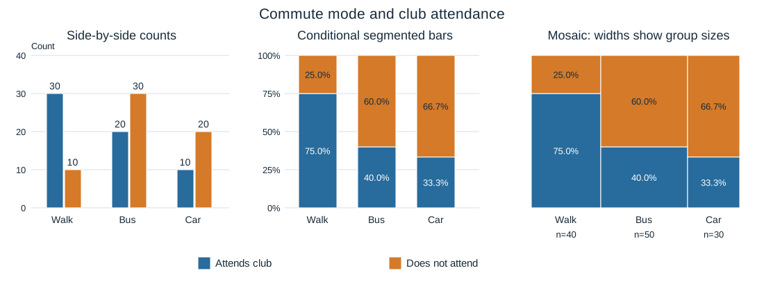
Each student has exactly one commute mode and one club-attendance label. This table and its three graphs describe all 120 surveyed students.
Part a
Compare the table with the side-by-side graph. Identify what the entries and bar heights represent; give one matching numerical example. Explain how a relative-frequency table would differ from the count table.
The table cells and grouped bar heights are counts of students with both labels. For example, 30 walkers attend a club in both displays. A joint-relative-frequency table divides every cell by 120, so that cell becomes .25; it displays proportions rather than counts without changing the observations.
| Evidence for credit | Points |
|---|---|
| Identifies counts and an accurate table/graph match. | 1 |
| Explains dividing by the full 120 for a joint-relative-frequency table. | 1 |
Part b
Compare the segmented bars and mosaic with the side-by-side graph. What reference group is 100% in each segmented bar? Explain both mosaic height and width, and identify information that equal-width segmented bars hide.
Each segmented bar is the students in one commute group: 40 walkers, 50 bus riders, or 30 car riders. Heights show conditional attendance proportions .75, .40 and 1/3. Mosaic segment heights show the same proportions, while widths are 40/120, 50/120 and 30/120. Equal-width segmented bars hide these unequal group sizes; count bars and mosaic widths retain them.
| Evidence for credit | Points |
|---|---|
| Names the three conditioning groups and correct conditional heights. | 1 |
| Explains mosaic width proportional to group size. | 1 |
| Contrasts count information with equal-height normalized bars. | 1 |
Part c
Compare the club-attendance distributions across commute modes using the table and the graphical views. Determine whether the variables are associated in these data, and explain the evidence.
Club attendance is 30/40=.75 for walkers, 20/50=.40 for bus riders and 10/30≈.333 for car riders. These different conditional distributions, visible in the segmented bars and mosaic heights, show association between commute mode and club attendance in this survey. The table provides the matching counts and denominators.
| Evidence for credit | Points |
|---|---|
| Compares all three conditional distributions with numbers. | 1 |
| Connects table and graphs to a contextual association conclusion. | 1 |
Justify a Claim About Club Attendance: worked answer
| Club attendance | Walk | Bus | Car | Total |
|---|---|---|---|---|
| Attends | 30 | 20 | 10 | 60 |
| Does not attend | 10 | 30 | 20 | 60 |
| Total | 40 | 50 | 30 | 120 |
Each student has exactly one commute mode and one club-attendance label. This table and its three graphs describe all 120 surveyed students.
Part a
Evaluate this claim: “Club attendance has the same distribution in every commute group because 60 students attend and 60 do not.” Justify your decision using specific evidence from both the table and at least one graph, identifying the relevant variables and groups.
The claim is unsupported. The equal marginal totals do not make the conditional distributions equal. The table gives attendance 30/40=.75 for walkers, 20/50=.40 for bus riders and 10/30≈.333 for car riders. The segmented bars or mosaic heights show the same unequal attendance shares. Thus attendance distribution differs by commute mode among these surveyed students despite the overall 60/60 split.
| Evidence for credit | Points |
|---|---|
| Rejects the claim with correct conditional numerical evidence. | 1 |
| Uses both table and a named graph. | 1 |
| Connects the unequal distributions to the surveyed commute/attendance variables rather than marginal totals alone. | 1 |