3.2 Probability Rules
Section Overview
- Interactive 3.2.1 - Example 3.2.1
- Example 3.2.1
- Example 3.2.2
- Gallery 3.2.1 - Venn Diagrams
- Interactive 3.2.2 - Example 3.2.2
- Example 3.2.3
- Interactive 3.2.3
- Pop Quiz 3.2.1
Probability Models
The idea of probability rests on the fact that chance behavior is predictable in the long run. Do we always need to repeat a chance process many times to determine the probability of a particular outcome? Fortunately, the answer is no.
A chance process is made up of two basic parts:
-
The sample space , the set of all possible outcomes which can be seen in Interactive 3.2.1 for rolling two die.
-
A probability for each outcome
Both of these comprise the probability model.
Interactive 3.2.1 Example 3.2.1
Example 3.2.1 — recorded answer
There are 36 possible outcomes when we roll two dice. Interactive 3.2.1 displays these outcomes. They make up the sample space . If the dice are well-made (fair), all 36 outcomes will be equally likely. That is, each of the 36 outcomes will come up on of all rolls in the long run. So each outcome has probability .
A probability model does more than just assign a probability to each outcome. It allows us to find the probability of any collection of outcomes, which we call an event. Events are usually designated by capital letters, like A, B, C, and so on.
That brings up to several basic probability rules:
-
For any event ,
-
If is the sample space in a probability model,
-
We also have several slightly more advanced rules:
-
Complement Rule:
-
Addition Rule for Mutually Exclusive Events: If A and B are mutually exclusive,
Two-Way Tables and Probability
When we’re trying to find probabilities involving two events, a two-way table can display the sample space in a way that makes probability calculations easier.
Example 3.2.2 — recorded answer
We’ll define events A: is male and B: has a tattoo
a) Since each of the 188 students in the class is equally likely to be chosen, and there are 23 students with a tattoo, .
b) We want to find , that is the intersection of the two events or . Looking at the intersection of the “Male” row and the “Yes” column, we see that there are 8 males with a tattoo. So .
c) This time, we’re interested in , that is the union of the two events or, . From the two-way table, we see that there are 97 males in the class, so . Can we just add to to get the correct answer? No! These two events are not mutually exclusive, since there are 19 males with a tattoo.
which is clearly wrong, since the probability is smaller than 1! From the two-way table, we see that there are students who are male or have a tattoo.
So .
We can also get this probability from subtracting the probability of the complement from 1. In other words:
The previous example revealed that we can’t use the addition rule for mutually exclusive events unless the two events have no outcomes in common. If events A and B are not mutually exclusive, they can occur together. The probability that one or the other occurs is then less than the sum of their probabilities.
This intuitive result is known as the general addition rule. That is, if A and A are any two events result from some chance process, then
Venn Diagrams and Probability
Venn diagrams are a great tool for illustrating the events within the sample space of a chance process. Gallery 3.2.1 gives further clarification to the following concepts and notation:
Gallery 3.2.1 Venn Diagrams
Frame 1 of 4
Aᶜ. It is the same as saying “The complement of A” or “Everything except A”. It includes all of the outcomes in the sample space not present in event A. Open full-size image S0221Frame 2 of 4
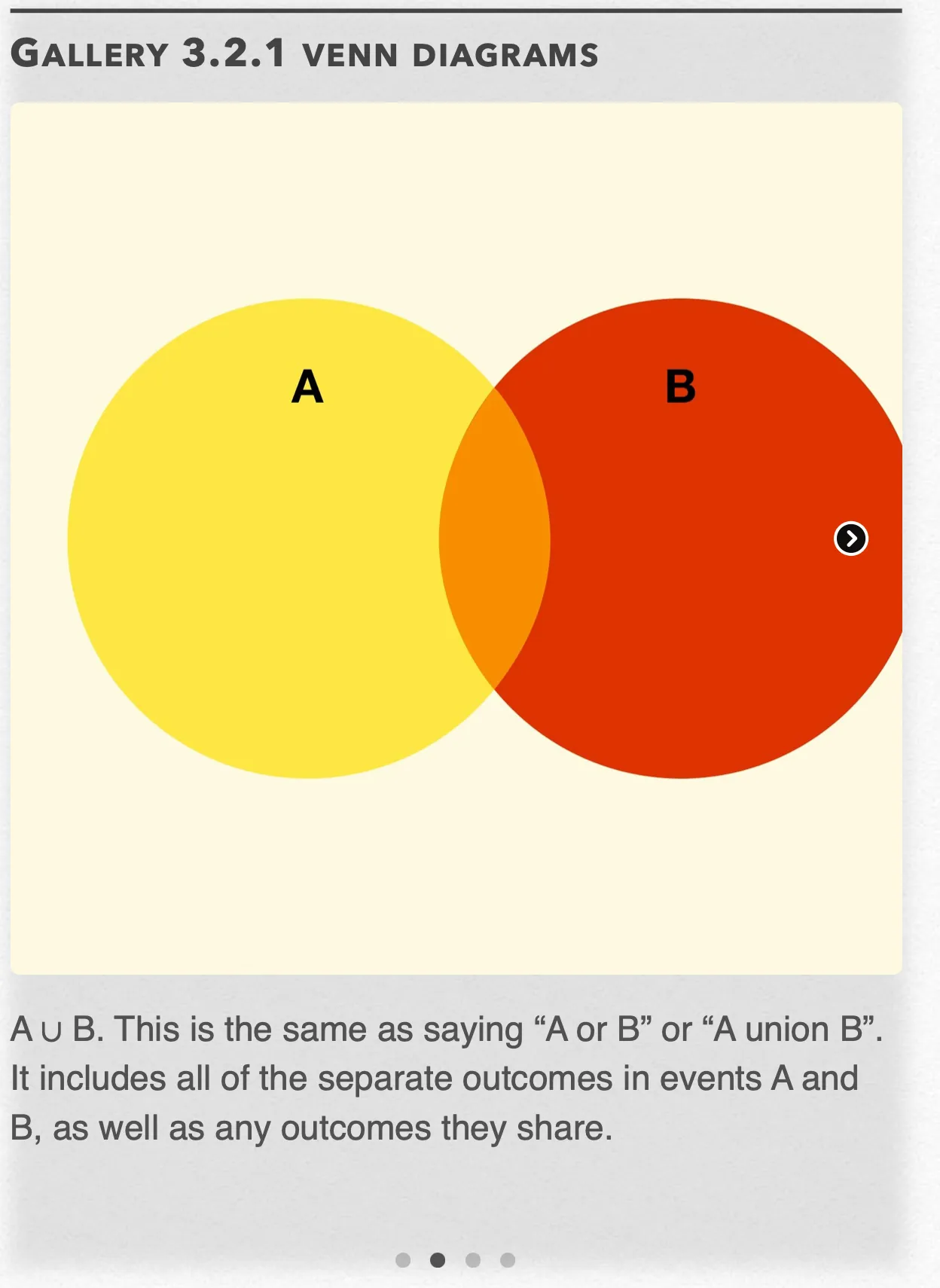
A ∪ B. This is the same as saying “A or B” or “A union B”. It includes all of the separate outcomes in events A and B, as well as any outcomes they share. Open full-size image S0222Frame 3 of 4
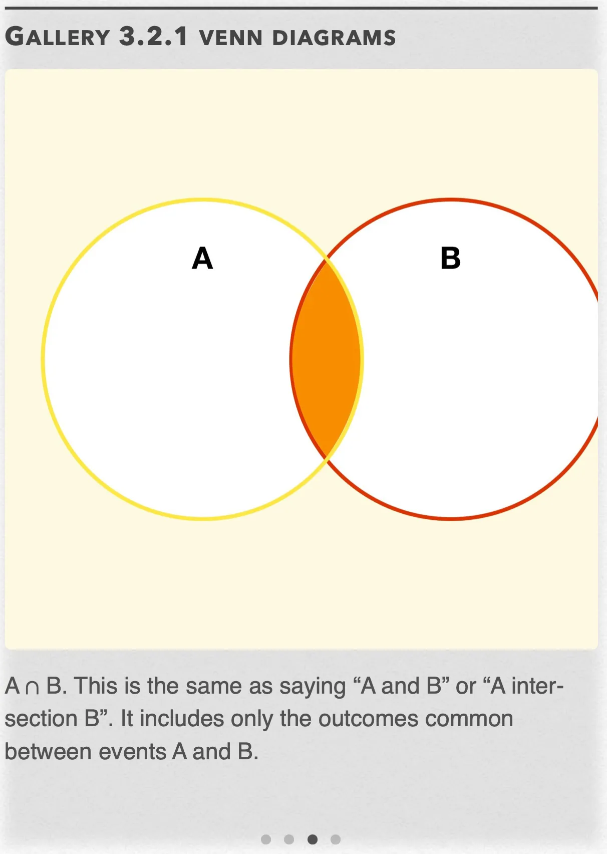
A ∩ B. This is the same as saying “A and B” or “A intersection B”. It includes only the outcomes common between events A and B. Open full-size image S0223Frame 4 of 4
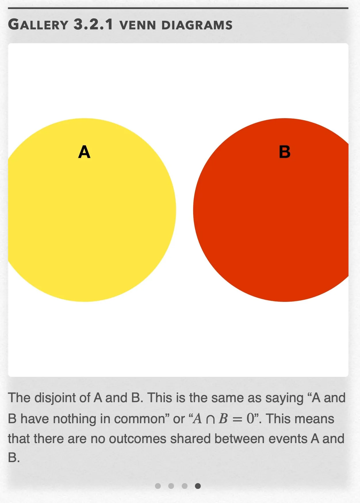
The disjoint of A and B. This is the same as saying “A and B have nothing in common” or “A ∩ B = 0”. This means that there are no outcomes shared between events A and B. Open full-size image S0224
Capture provenance
Filename capture times, with no recorded timezone. Frames above follow the original gallery positions.
- · S0221 · displayed frame 1
Screenshot 2026-10-05 at 3.51.53 PM.png - · S0222 · displayed frame 2
Screenshot 2026-10-05 at 3.51.58 PM.png - · S0223 · displayed frame 3
Screenshot 2026-10-05 at 3.52.02 PM.png - · S0224 · displayed frame 4
Screenshot 2026-10-05 at 3.52.06 PM.png
The gallery notation, as recorded: .
Interactive 3.2.2 Example 3.2.2
A ∩ Bᶜ — recorded annotation
This represents males without a tattoo
Aᶜ ∩ B — recorded overlap annotation
This represents males with a tattoo.
Aᶜ ∩ B — recorded right-region annotation
This represents females with a tattoo
Aᶜ ∩ Bᶜ — recorded annotation
This represents females with no a tattoo.
What is Conditional Probability?
Suppose we know that event A has happened. Then the probability that event B happens given that event A has happened is denoted by . This is known as conditional probability.
For the pierced-ears scenario, however, . When knowledge that one event has happened does not change the likelihood that another event will happen, we say that the two events are independent.
Tree Diagrams and Probability
If you toss a fair coin three times, what’s the probability that you get two heads? By the reasoning we’ve already established, it’s the proportion of times you would get “HH” if you tossed the coin three times over and over again. Since there is only one way to get two heads, and there are possible outcomes, the probability is .
This idea of multiplying along the branches in a tree diagram leads to a general multiplication rule for finding the probability that two events happen together:
Example Problem 3.2.3 — recorded answer
The percents of each group who play first person shooters are conditional probabilities. We want to find the unconditional probability . Making a tree diagram should help.
To get the probabilities at the far right, we used the general multiplication rule and multiply the unconditional (original) probabilities with the conditional probabilities:
For instance, the probability that a randomly chosen internet user is an 18- to 30-year old who plays first person shooters is
This probability appears at the end of the topmost branch.
There are three disjoint paths to “shooter yes,” one for each of the three age groups. These paths are shown in Interactive 3.2.3. Because the three paths are disjoint, the probability that an adult internetr plays first person shooters is the sum of their probabilities:
Interactive 3.2.3 Example 3.2.3
The branch probabilities visible in the original diagram:
| Age group | Original probability | Shooter YES | Shooter NO |
|---|---|---|---|
| 18–30 years | 0.57 | 0.5 | 0.5 |
| 31–40 years | 0.35 | 0.51 | 0.49 |
| 41+ years | 0.08 | 0.16 | 0.84 |
Pop Quiz 3.2.1
Glossary and deeper reading · 9 refreshers
These editorial refreshers supplement the reading. Definitions and examples are added guidance; original source wording and recorded answers remain in their original context.
-
Probability
Probability quantifies how likely an event is under a specified chance model. It lies between 0 and 1, with larger values representing greater likelihood. For example, drawing a red card from a well-shuffled standard deck has probability one half.
-
Sample space
The sample space is the set of all possible outcomes of a chance process. Outcomes must be described at the level relevant to the question being modeled. For example, the sample space for one draw from a red-blue bag can be red and blue.
-
Event in probability
An event is a set of outcomes from a chance process’s sample space. The event occurs when the observed outcome belongs to that set. For example, rolling an even result is the event containing 2, 4, and 6 for a six-sided die.
-
Two-way table
A two-way table organizes counts for combinations of two categorical variables. The cells show combinations, while row and column totals summarize each variable separately. For example, a table can classify students by grade level and whether they walk to school.
Read more: Two-way table in the captured Statistics reading →
-
General addition rule
The general addition rule finds the probability that at least one of two events occurs. It adds their probabilities and subtracts the probability that both occur, avoiding double counting. For example, the probability of a card being red or a king must subtract the red kings counted twice.
-
Mutually exclusive events
Mutually exclusive events cannot occur together in the same trial. Their intersection is empty, so the probability that either occurs is the sum of their probabilities. For example, rolling exactly 1 and rolling exactly 4 are mutually exclusive outcomes of one die roll.
-
Venn diagram
A Venn diagram represents sets or events with regions inside a sample-space boundary. Overlapping regions show outcomes shared by two events. For example, overlapping circles for red cards and kings identify the red kings.
-
Tree diagram
A probability tree represents successive stages of a chance process using branches. Multiplying the relevant conditional probabilities along a path gives that path’s probability. For example, a two-draw tree can show how a bag’s second-draw probabilities change when the first item is not replaced.
-
General multiplication rule
The general multiplication rule finds the probability that two events both occur. It multiplies the first event’s probability by the second event’s probability conditional on the first. For example, two red draws without replacement use the updated red proportion for the second draw.