2.11 Normal Models: Areas, Cutoffs and Relative Position

A Smooth Model for a Measured Quantity

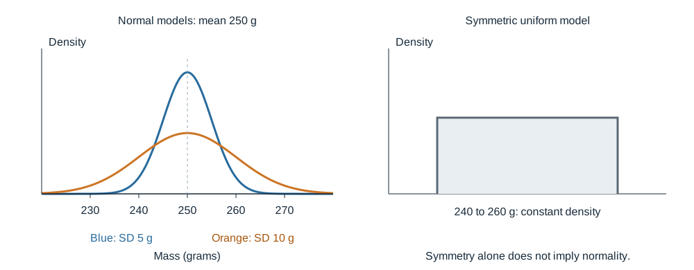
The mass of a coffee bag is a measurement, not a count. Within a measurement domain it can take intermediate values such as 249.6 g or 249.63 g. A continuous random variable can take any value within its specified domain, and intervals have probabilities. A normal curve is a useful approximation for many such variables, but it is not the model for every continuous or symmetric distribution.

A normal distribution is continuous, unimodal, bell-shaped and symmetric. It can model the distribution of observed data, and it can model probabilities for a continuous random variable representing a new observation. The curve has two parameters: its mean μ sets the center; its SD σ controls its width and height. With the same mean, smaller σ makes a taller, narrower curve; larger σ makes it shorter and wider. Each complete curve has area 1.

Worked Example: Parameters and Standard Normal

Suppose a supplied fill-mass model has mean 250 g and SD 5 g. Its one-SD marks are 245 and 255 g: the center is their midpoint, and the SD is the distance from the center to either mark. These are model parameters, not an observed sample mean and sample SD.

The standardized variable is $Z=(X-250)/5$. Its mean is $(250-250)/5=0$, and its SD is $5/5=1$. It therefore has the standard normal distribution, whose mean is 0 and SD is 1. Z has no gram units. This normal standardization is useful for areas; it does not require a general theory of combining arbitrary random variables.

Approximate Areas at One, Two and Three SDs

The empirical rule, or 68–95–99.7 rule, gives approximate percentages in a normal model: 68% within one SD of the mean, 95% within two, and 99.7% within three. For these coffee bags the intervals are 245–255 g, 240–260 g and 235–265 g. Symmetry splits a central region equally at the mean and splits its outside area into equal tails.

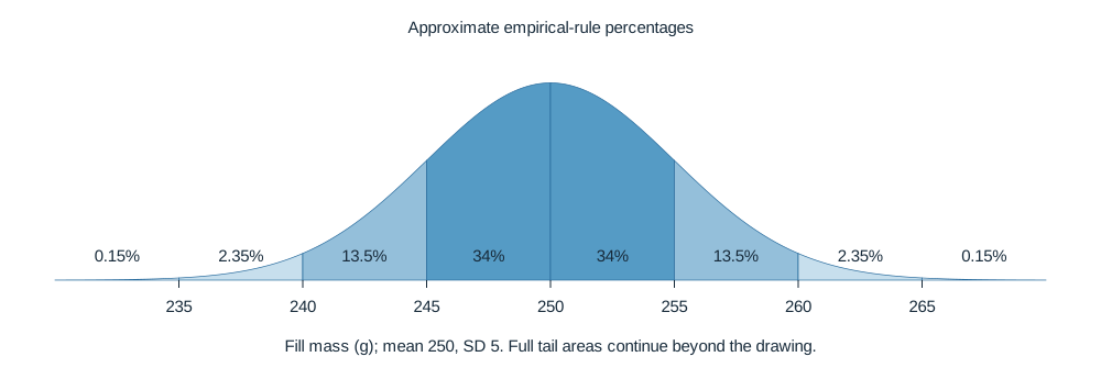
For example, 250–255 g contains about 34%. The band 255–260 g contains $(95-68)/2=13.5\%$, and above 260 g is about $(100-95)/2=2.5\%$. These are approximations, not exact normal-CDF results.

Calculate an Area from Given Bounds

If X is approximately normal, its probability within an interval is the curve area above that interval. The total area is 1. Let $\Phi(z)=P(Z\le z)$ denote standard-normal left-tail area. Standardize each boundary and subtract left-tail areas for an interval.

For the supplied coffee model, below 245 g has z=−1 and probability about 0.158655. Above 260 g has z=2 and probability $1-\Phi(2)\approx0.022750$. Between 240 and 257 g has boundaries z=−2 and z=1.4:

About 89.65% of model-bags lie in that mass interval. A continuous normal model assigns probability 0 to one exact value; changing strict to inclusive endpoints does not change its area. This is different from a discrete distribution, where including a boundary can add positive probability. The ideal normal model extends along the real axis; its use for physical masses is an approximation near the relevant positive values, not a claim that negative masses occur.

Find Bounds from a Percentage

Now reverse the question. The lowest 10% has left-tail area 0.10 and standard-normal cutoff about −1.28155. Transform back: $x=250+5(-1.28155)\approx243.592$ g. The highest 10% starts at about 256.408 g because its left-tail area is 0.90. A central 80% interval leaves 10% in each tail and uses those same two boundaries.

An inverse-normal tool can find the cutoff directly from area, mean and SD. A standard-normal table can instead find z whose left area is closest to the target; then use $x=\mu+\sigma z$. Always identify whether the stated percentage is a left, right, central or two-tail area before using either method.

For a percentage number p between 0 and 100, lower bound $x_a$ and upper bound $x_b$, the interval statements are:

These describe lowest-p%, between-bounds-p%, and highest-p% regions respectively. They are alternative region types, not three claims about one fixed pair of bounds.

The most extreme p% on both sides splits that percentage equally:

For the most extreme 10%, each tail is 5%, using z≈±1.64485. The coffee-model bounds are about 241.776 and 258.224 g; the extreme event is below the lower bound or above the upper bound. Do not put 10% in each tail—that would make 20% extreme overall.

Compare with Percentiles and Proportions

Raw values from different models may not be directly comparable. A 254 g bag in the mean 250/SD 5 model has z=.8 and percentile about 78.81. A 508 g bag in a separate mean 500/SD 12 model has z≈.667 and percentile about 74.75. The first reading is higher relative to its own model despite its smaller raw mass. About 21.19% of the first model lies above 254 g, compared with 25.25% of the second above 508 g.

Percentiles and above/below proportions let us compare relative position within one normal model or between models. State the model and area direction along with the number. A z-score supports the area calculation, but the percentile or proportion explains how much of the modeled population is below or above the observation.

Try It Yourself

The following original practice applies the ideas above to a fresh setting. Show the reasoning requested in each part. Answers and task-specific rubrics are on the separate solutions page.

Original generated practice for the Fall 2026 course.

Describe and Calculate Normal-Model Parameters

Model Q is a normal model for repeated temperature readings in °C. Its center is marked 75, and its one-SD marks are 71 and 79. Model R is also normal, centered 75 with one-SD marks 67 and 83. A separate model U is uniform on 65–85°C, with constant density over that interval and zero elsewhere. The markings describe supplied model parameters, not observed sample summaries.

Part a

Describe Q and R as continuous distributions, including unimodality, bell shape, symmetry and the effect of their differing spread on curve width/height. Explain how a normal curve can model both a histogram of many readings and the probability distribution of a new reading. Contrast U: explain its continuous domain and why symmetry alone does not make it normal.

Your reasoning

Part b

Calculate the mean and SD of Q and R from the marked intervals. For Q define Z=(Q−75)/4 and calculate its mean and SD. Name this resulting normal distribution and state whether its standardized readings retain °C units.

Your reasoning

Worked answer and rubric

Use the Empirical Rule for Commute Time

A supplied normal commute-time model has mean 50 minutes and SD 6 minutes. Use empirical-rule approximations rather than exact normal-CDF values. One-, two-, and three-SD boundaries must be calculated from the model.

Part a

Calculate the three central intervals within one, two and three SDs and their approximate percentages. Identify both names of the rule you use.

Your reasoning

Part b

Calculate the approximate percentages between 50 and 56, between 56 and 62, above 56, below 32, and outside 38–62. Explain the symmetry and subtraction for each; label the regions on a sketch or give their bound/area descriptions.

Your reasoning

Worked answer and rubric

Calculate Normal Battery-Life Areas

A supplied approximately normal model for a battery population has mean 12 hours and SD 1.5 hours. Let X be one battery’s life. You may use normal technology or the following standard-normal left-tail values: Φ(−1)=.158655, Φ(2)=.977250, Φ(−2/3)=.252493 and Φ(4/3)=.908789.

Part a

Calculate P(X<10.5), P(X>15), and P(11<X<14). For each, standardize the bounds, identify the shaded region or describe it with labeled bounds, and show the area calculation.

Your reasoning

Part b

Interpret the interval probability for the stated battery population. State the full curve’s probability/area and explain whether including the exact endpoints changes these continuous-model probabilities.

Your reasoning

Worked answer and rubric

Find Normal Cutoffs and Extreme Tails

A supplied normal phone-use model has mean 10 hours and SD 2 hours. For an area expressed as a percentage number p, use p/100 as a probability. Supplied standard-normal quantiles are Φ⁻¹(.05)=−1.6448536, Φ⁻¹(.10)=−1.2815516, Φ⁻¹(.90)=1.2815516 and Φ⁻¹(.95)=1.6448536. Use these values as a table, or equivalent inverse-normal technology; explain which left-tail area you select.

Part a

Find the upper boundary x_a of the lowest 10% and write the corresponding probability inequality using p/100. Show the selected standard-normal area and the conversion to hours.

Your reasoning

Part b

Find the lower boundary x_b of the highest 10% and write its strict probability inequality. Explain why the inverse input is .90 rather than .10.

Your reasoning

Part c

Find both bounds of the central 80% interval. Identify p, lower bound and upper bound, and write P(x_a<X<x_b)=p/100. Verify the area by subtracting the two left-tail areas.

Your reasoning

Part d

Find the most extreme 10% on both sides. State each tail area as one-half times p/100, calculate both cutoffs and write both strict tail inequalities. Explain why using 10% in each tail would answer a different question.

Your reasoning

Worked answer and rubric

Compare Relative Positions Within and Between Models

For the within-model comparison, Model A is normal for fill mass with mean 250 g and SD 5 g; its two readings are 254 g and 247.5 g. For the separate between-model comparison, Model C is normal with mean 300 g and SD 8 g, with a reading of 309.6 g; Model D is normal with mean 400 g and SD 10 g, with a reading of 413 g. All are supplied population models. Standard-normal left-tail values: Φ(.8)=.788145, Φ(−.5)=.308538, Φ(1.2)=.884930 and Φ(1.3)=.903200.

Part a

Calculate the percentiles of both Model A readings and compare their relative positions within that distribution. Also calculate the proportions above each reading and connect the two comparisons.

Your reasoning

Part b

Compare 309.6 g in Model C with 413 g in Model D using percentiles and proportions above the readings. Show the standardized positions and area calculations. Explain why comparing only raw grams or reporting only z-scores would not complete the requested comparison.

Your reasoning

Worked answer and rubric