Scatterplots: Preserve, Describe, and Defend the Pattern

Two numerical measurements on the same individual tell a story that two separate lists cannot. A scatterplot keeps the pairing visible. Its purpose is to show how values of one variable tend to accompany values of the other, including exceptions to the pattern.

Keep the Pairs

A bivariate quantitative data set contains ordered pairs from two quantitative variables, collected from the same individuals in a sample or population. Suppose five students each study a word list for a recorded number of minutes and then complete the same recall activity. Each row below is one student’s pair; it is not permissible to sort the two columns separately and invent new pairs.

Student	Study time, x (minutes)	Words recalled, y (count)
A	0	5
B	10	8
C	20	10
D	30	14
E	40	16

The explanatory variable is placed on the horizontal x-axis. It is the variable used to explain or predict the corresponding response. The response variable is placed on the vertical y-axis. Here, study time explains or predicts recall count; recalling five words is not a fifth minute of study. Axis labels must identify both variables and their units.

Worked Example: Construct the Plot

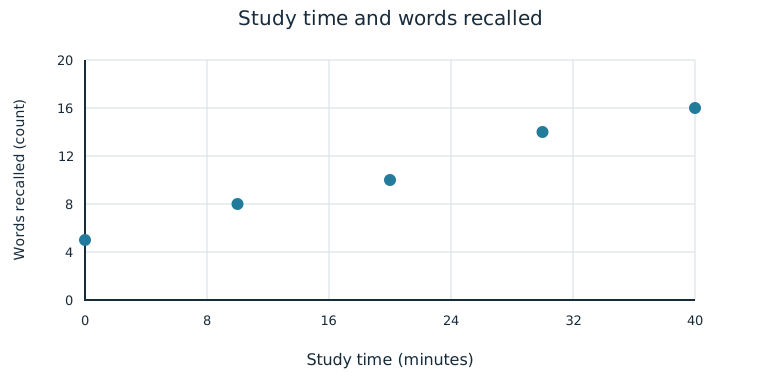
Choose scales that include every observation: 0–40 minutes horizontally and 0–20 words vertically. For student B, move to x=10 minutes and y=8 words, then place one point. Repeat for all five ordered pairs. Do not draw a bar for each student or a line that claims a time sequence. Scatterplot points need not be joined.

Describe the Association

Describe form, direction, strength, and unusual features. Form may be linear or non-linear if a pattern exists. A linear pattern follows an approximately straight path; a non-linear pattern bends. Direction may be positive or negative: in a positive association, response values tend to increase as explanatory values increase; in a negative association, they tend to decrease. An association says “tend to,” rather than promising the same result for every individual.

Strength describes how closely points follow the general pattern. Strong points cluster closely around that pattern; moderate points have more scatter; weak points have substantial scatter. Strength is judged relative to the pattern, which may itself be curved. A steep slope alone does not make an association strong. An unusual feature may be a cluster of individuals or an individual point that does not fit the general pattern.

For the recall plot, the form is approximately linear, the direction is positive, and the points follow the pattern closely. There is no obvious isolated point or separate cluster. A useful sentence is: “For these five students, longer study times are associated with larger recall counts in a strong, approximately linear pattern.” The context and observed group are part of the description.

Worked Comparison: A Curve

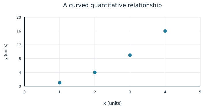
The pairs (1,1), (2,4), (3,9), and (4,16) trace an upward curve rather than a straight line. Their association is positive and strong, but non-linear. A description that says only “strong positive” leaves out the form; a line is not automatically appropriate because the points follow some pattern closely.

Justify a Graphical Claim

A scatterplot can support a claim about the relationship between two numeric variables. State the claim, cite a relevant feature of the plotted observations, and explain how the feature bears on that claim. For example, the student with 10 minutes of study recalls 8 words, while the student with 30 minutes recalls 14; the other points follow the same general upward pattern. These comparisons support a positive association in this observed group.

One favorable pair is weaker evidence than a pattern across the plot. An exceptional point can limit a claim that every individual follows a rule. The plot also does not, by itself, tell how the students were selected or whether study times were randomly assigned. A visual relationship should not silently become a cause-and-effect conclusion. The independent practice asks you to construct and defend your own description from complete paired observations.

Independent Practice

Use the information in each question to make your own calculation, representation, or argument. Explain what your result means in its setting.

Original generated practice for the Fall 2026 course.

Two measurements, one student

A club records each member’s weekly practice time in hours and target score in points. Member R has the pair (3,18).

Part a

Identify the two quantitative variables, what one ordered pair represents, and which variable belongs on each axis if practice time is used to predict score. Explain why matching the hours of one member with another member’s score would be invalid.

Your reasoning

Worked answer and rubric

Place every observed pair

Four generated observations are (x,y)=(1,7),(2,6),(3,4),(4,3), where x is distance from a lamp in meters and y is light reading in instrument units.

Part a

Construct a scatterplot of all four pairs. Label axes and units, use consistent scales, and show four distinct points. Describe the direction of the pattern.

Your reasoning

Worked answer and rubric

Strong does not mean straight

The complete generated pairs are (1,1),(2,4),(3,9),(4,16).

Part a

Describe the form, direction, strength, and unusual features of this scatterplot. Explain why “strong positive linear” is an incomplete or inaccurate description.

Your reasoning

Worked answer and rubric

A claim about the observed students

Five students have the pairs (study minutes, words recalled)=(0,5),(10,8),(20,10),(30,14),(40,16).

Part a

Justify or reject this claim: “In this observed group, longer study times are associated with larger recall counts.” Cite the plotted pattern and at least two numerical pairs.

Your reasoning

Worked answer and rubric

Practice time, clusters, and an exception

A coach observes seven club members. Practice time is used to explain score; no practice times were randomly assigned. The generated data below are complete.

Seven club members: each row preserves one member’s two measurements

Member	Practice (hours)	Target score (points)
1	1	12
2	2	14
3	3	16
4	8	26
5	9	28
6	10	30
7	2	29

Part a

Construct a scatterplot from the seven paired observations. Label both axes with their variables and units, choose consistent scales including all observations, and plot every member.

Your reasoning

Part b

Describe form, direction, and strength. Identify the two main clusters and the unusual observation, and explain how that observation affects your description.

Your reasoning

Part c

Justify or reject each claim using the plotted evidence: (i) the high-practice cluster generally has higher scores; (ii) every member practicing fewer than 4 hours scores fewer than 20 points.

Your reasoning

Worked answer and rubric