Errors and Power: Detecting a Difference Without Claiming Certainty

These lessons and problems are newly written for the revised course. Worked examples show complete reasoning; the application questions ask you to make and defend your own choices.

Separate the truth from the decision

Imagine deciding whether a food shipment’s contamination proportion exceeds an acceptable baseline. A test decision is based on a sample, so even a well-designed procedure can be wrong. A Type I error rejects a true null: the small p-value suggests an alternative that is actually false. A Type II error fails to reject a false null: the p-value is not small, yet a real population difference exists. The same phrases become meaningful only after naming the population truth and the practical decision.

Two possible truths and two possible decisions

Population truth	Reject the null	Fail to reject
Null true	Type I: false alarm	Correct decision
Specified alternative true	Correct detection	Type II: missed difference

PowerEditorial qualification: The captured text describes power as detecting a Type II error. Power is the probability of correctly rejecting the null hypothesis for a specified true alternative, equal to 1 − β. is the probability of correctly rejecting a false null at a specified population alternative. It is not a probability that the null is false in today’s study. One sample’s result does not determine the population truth, and failure to reject must not be called accepting or proving that truth.

A corrected, fully specified packet-mass model

The following new modeling information makes a complete probability calculation possible: packet masses are independently drawn from a Normal population with known σ=0.010 kg, n=5, target μ₀=18.000 kg. This supplied probability model illustrates power; the required mean-inference method elsewhere uses t when population σ is unknown. The standard deviation of the sample mean is σ/√n=0.00447214 kg, not σ/n. A two-sided rule rejects when x̄ lies outside 18.000±1.96(0.00447214), so its failure-to-reject interval is [17.9912346,18.0087654] kg.

Under the target mean the false-alarm probability is 2P(Z>1.96)≈0.05. This is α: reject probability conditional on a true null. Now assume the population mean is actually 18.015 kg. The same boundaries standardize to approximately −5.31410 and −1.39410 under that shifted population. The Type II probability is the area between these boundaries under the shifted sampling distribution.

Thus about 8.16% of repeated checks miss this particular shift, while about 91.84% detect it. The small left-boundary probability must be subtracted, even though it is nearly zero. Labeling 0.0816 as power reverses the meaning. Both β and power are conditional on μ=18.015; α is conditional on μ=18.000. Change the true mean and the detection probability can change.

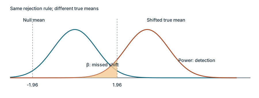
Four ways to make detection easier

For a given test and specified alternative, low Type II probability means high power: for example, β=0.20 corresponds to power=0.80. Holding other relevant settings fixed, power increases when sample size increases, standard error decreases, the true parameter is farther from the null, or significance level α increases. These relationships describe a probability procedure, not a promise about an individual sample. Sample size and standard error are connected: increasing n commonly helps by reducing SE.

Consider the supplied one-sided model that rejects Z>1.644854 at α=0.05. Under a true standardized effect θ/SE, power=Φ(θ/SE−1.644854). With θ=0.15 and SE=0.10, power≈0.4424. Doubling n reduces SE to 0.10/√2, giving power≈0.6831. Reducing measurement variability at the original n so SE=0.08 gives ≈0.5910. Moving the true parameter to 0.25 at original SE gives ≈0.8038. Raising α to 0.10 lowers the critical threshold to 1.281552 and gives ≈0.5865. Each calculation compares a stated alternative and design; the sample-size change acts through SE rather than pretending both can vary independently.

Higher confidence in an interval uses a larger critical multiplier, while higher α in a test makes rejection easier. Keep these two “higher” settings separate: they refer to different procedure goals.

Use consequences before collecting data

In the food-shipment setting, a false alarm can destroy safe food; a missed contaminated shipment can expose customers. Type II consequences may dominate there. In another setting, such as a costly medical follow-up triggered by an exploratory screen, a false alarm may deserve more emphasis. Compare both consequences before designing the study; there is no universal more-serious error.

Because α is the Type I probability, false-alarm consequences guide its choice. Lowering α reduces false rejection under the null but usually lowers power at a fixed alternative and sample size. Because n affects Type II probability, sample-size planning can improve the chance of detecting a harmful effect while retaining a cautious α. Better measurement precision may also help. Cost, feasibility, the smallest consequential difference, and both kinds of error belong in that planning discussion. Power 0.83 at contamination p=0.04 means a 17% miss probability at that alternative; it does not assign 17% to every conceivable contaminated proportion.

Independent Application

Work through each investigation before opening the separate solutions. State parameters, show calculations and connect your reasoning to the actual study.

Original generated practice for the Fall 2026 course.

A complete power model for packet mass

This newly specified packet-mass model samples five packets independently from a Normal population with known SD 0.010 kg. Target mean is 18.000 kg. A two-sided rule rejects if sample mean is below 17.9912346 or above 18.0087654 kg, equal to 18.000±1.96(0.010/√5). The sample-mean SD is σ/√n. For a true mean 18.012 kg, the standardized acceptance endpoints are -4.6432816 and -0.7232816; their normal CDF values are 0.000001715 and 0.234753456. Under the null Φ(1.96)=0.975002105. This supplied probability model illustrates power and does not add a required unknown-σ mean method.

Part a

Define a Type I error and Type II error in this context, and explain the actual true mean and decision involved in each. State what power measures.

Your reasoning

Part b

Recompute the standard deviation of the sample mean and both acceptance boundaries from the model. Find the Type I probability under the target and the Type II probability and power when μ=18.012. Show the interval probability before taking the complement.

Your reasoning

Part c

Interpret β and power in repeated quality checks. Explain why reversing these two labels or calling failure to reject “accepting a true target” would misstate the result.

Your reasoning

Worked answer and rubric

False alarms and missed contamination

A food-testing agency treats a shipment’s population contamination proportion p=0.02 as the baseline and tests Hₐ:p>0.02 with a prespecified valid procedure. At the baseline its rejection probability is 0.01. At a harmful proportion p=0.035 its power is 0.76. Rejecting a safe shipment destroys it; failing to flag a contaminated shipment can expose customers. A proposed research change lowers α while leaving sample size, variability, and the harmful alternative fixed. Another proposal increases sample size at the same α.

Part a

Describe the two possible errors using the shipment decisions and population truth. Calculate the Type I probability, the Type II probability at p=0.035, and the probability of detecting that harmful alternative. Explain why the 0.24 Type II probability cannot be attached to every possible contaminated proportion.

Your reasoning

Part b

Explain which error may have more serious consequences here, and how that judgment should affect planning before data collection. Describe the consequences of lowering α at fixed n and increasing n at fixed α; address both Type I and Type II concerns.

Your reasoning

Worked answer and rubric

Which design has the best chance to detect a shift?

A supplied one-sided Normal sampling model tests θ=0 versus θ>0. At true θ, the standardized statistic has mean θ/SE and SD 1; reject when Z>c. At α=.05 c=1.644854; at α=.10 c=1.281552. Baseline: θ=.12, SE=.10. A doubles n so SE=.10/√2. B reduces population variability at original n so SE=.08. C uses true θ=.22 at original SE. D uses α=.10 at original θ/SE. All other stated settings stay fixed. Use power=Φ(θ/SE−c). For computation: Φ(-0.4448540)=0.32821263; Φ(0.0522023)=0.52081624; Φ(-0.1448540)=0.44241307; Φ(0.5551460)=0.71060260; Φ(-0.0815520)=0.46750149.

Part a

Calculate baseline power and Type II probability, then calculate power and Type II probability for A–D. Identify the relevant factor in each comparison, and explain in words how it makes correct rejection more likely. Explain why sample size and standard error are linked mechanisms.

Your reasoning

Part b

A teammate says “The largest power guarantees the null is false, and increasing α is always the best choice.” Assess both claims and choose a defensible design change if false alarms are expensive.

Your reasoning

Worked answer and rubric