Estimating a Proportion: Confidence, Precision and a Population Claim

These lessons and problems are newly written for the revised course. Worked examples show complete reasoning; the application questions ask you to make and defend your own choices.

The sample gives an estimate, not the whole population

A school wants to know what proportion of its enrolled students prefer a new breakfast menu. Asking every student may be impractical, but a carefully chosen sample can estimate the population response. The unknown parameter p is the proportion of all enrolled students who prefer the proposed breakfast menu. That definition includes the numerical kind of parameter, the response and the population. A sample proportion p̂ is calculated from the observed sample; it changes when another sample is selected.

A confidence interval is an interval estimate for a population parameter. For one binary response from one randomly selected sample, use a one-sample z-interval for a population proportion. It begins with the sample proportion as a point estimate and adds a margin for sampling variation. The interval estimates p; it does not predict which particular students prefer breakfast or put individual yes/no responses into a numerical interval.

In a new worked example, an SRS of 180 students is drawn without replacement from 4,000 enrolled students. Of those selected, 117 prefer the proposal. The point estimate is 117/180=0.65. Even if the procedure is sound, a different random sample could give a different p̂. Reporting only “65%” conceals that sampling uncertainty. Our goal is a range of plausible values for the population proportion, with a stated confidence method.

Check the design and the observed counts

Three checks justify the ordinary z-interval approximation. The data should come from a random sample. When sampling without replacement, verify n≤0.10N, equivalently N≥10n. Finally, both observed successes n p̂ and failures n(1−p̂) should be at least 10. The two count checks support a reasonably normal sampling-distribution approximation; random selection and the sampling fraction address different aspects of the design.

For the breakfast example, the SRS supplies randomization and 180≤0.10(4,000)=400 verifies the fraction. Observed successes are 117 and failures are 63, both at least 10. These are observed counts because the unknown p is being estimated. Substituting a convenient hypothetical p₀ changes the question and does not repair too few actual successes.

A voluntary website survey can have thousands of responses and still lack random selection. An SRS of 120 from only 900 people can have balanced successes and failures yet violate 120≤90. An SRS of 60 with just four successes can satisfy the design checks but fail the count condition. A complete justification uses the actual context and all three checks, rather than treating “large sample” as permission to calculate everything.

From standard error to endpoints

The standard error is an estimate of the standard deviation of the sampling distribution of a statistic. Here it estimates typical sample-proportion variation around the fixed population p. It is not the standard deviation of an individual yes/no response. Estimate it with the observed sample proportion, then multiply by a critical value to obtain a margin of error.

The critical value z* is chosen so that −z* and +z* enclose the central C% of the standard normal distribution. For approximately 95% confidence, z*=1.96. The breakfast sample gives SE=√[0.65(0.35)/180]≈0.0355512. Its margin is 1.96(0.0355512)≈0.0696804. Thus the interval is 0.65±0.0696804, approximately (0.5803196,0.7196804).

Worked breakfast interval

Quantity	Value	Meaning
Point estimate	0.6500	Observed preference proportion
SE	0.03555	Estimated repeated-sample proportion variation
MOE	0.06968	Extension from estimate to either endpoint
Full width	0.13936	Twice the margin of error

The lower endpoint is about 0.5803 and the upper about 0.7197. The full width extends in both directions; MOE is half that width. These units are proportions: the margin is about 6.97 percentage points, not a 6.97% relative increase in breakfast preference.

Interpret the range and the method separately

We are 95% confident that the population proportion of enrolled students preferring the breakfast proposal lies between about 0.5803 and 0.7197. This is a statement about p for the named school population. The range contains values we regard as plausible given the sample and procedure. Since its entire range exceeds 0.50, it supplies convincing evidence that a majority of enrolled students prefer the proposal.

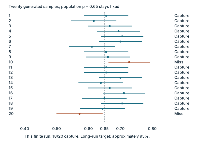
The confidence level describes the method: in repeated random sampling with the same sample size, approximately 95% of intervals constructed this way would capture the fixed population proportion. A particular computed interval either contains p or does not. It may miss, even though the method has 95% confidence; the statement does not mean p moves randomly among the endpoints or that 95% of students lie in that range.

The figure repeats the same sampling and calculation method in a generated population with known p=0.65. Knowing the simulation truth lets us identify captures and misses. In a real survey the unknown truth prevents us from labeling our one interval with certainty. A small finite run need not have exactly the advertised capture percentage.

If an otherwise valid interval were (0.47,0.63), both minority and majority values would be plausible. That interval would not give convincing evidence for a majority, and it would not prove a majority absent. Use the range to justify the actual investigative claim rather than attaching a conclusion mechanically to the word “confidence.”

Choose precision and confidence before sampling

For a fixed sample, greater confidence encloses more of the normal curve and needs a larger z*. Therefore the critical value, margin of error and interval width all increase. In the breakfast sample, the same SE≈0.0355512 gives margins about 0.05848 at 90% (z*=1.645), 0.06968 at 95% (1.96), and 0.09158 at 99% (2.576). A narrower interval from the same data cannot retain the same capture guarantee simply by changing the label.

At fixed confidence and comparable p̂, larger n reduces SE and tends to narrow the interval. The width is approximately proportional to 1/√n. Moving from n=180 to n=720 while retaining p̂=0.65 halves SE, margin and width. It does not quarter the width: four times the observations give only about twice the precision.

For planning, rearrange the MOE formula before data collection:

Suppose a town with 100,000 residents wants a 95% margin at most 0.03. A pilot estimate 0.65 gives planned n=1.96²(0.65)(0.35)/0.03²≈971.0711, so use at least 972. If a sample-proportion estimate is not defined or cannot be calculated, use 0.50. This maximizes p̂(1−p̂) at 0.25 and gives the conservative upper bound n≈1067.1111, hence 1,068. Always round up for a minimum-size requirement. Both proposed sizes meet the town sampling fraction, but the later realized data still need random selection and both observed-count checks. Planning is not evidence that a survey has already been completed.

Independent Application

Work through each investigation before opening the separate solutions. State parameters, show calculations and connect your reasoning to the actual study.

Original generated practice for the Fall 2026 course.

How many students want the new lunch menu?

An SRS of 200 students is selected without replacement from 6,000 enrolled students. Of the sampled students, 120 prefer a proposed lunch menu to the current menu. Estimate the population preference proportion with 95% confidence; use z*=1.96. The school asks whether the interval supplies convincing evidence that a majority prefers the proposal.

Part a

Define the population parameter with the response and population. Select the interval procedure and justify all three conditions with the actual observed counts and sampling fraction.

Your reasoning

Part b

Calculate the point estimate, SE, MOE and endpoints. Describe what SE estimates and distinguish it from variability of individual yes/no responses. Explain what the critical value 1.96 bounds on the standard normal curve and why MOE is half the full interval width.

Your reasoning

Part c

Interpret the interval and the 95% confidence level separately. Use the endpoints to assess the majority claim, and explain why the interval does not say 95% of individual students lie inside a numerical range.

Your reasoning

Worked answer and rubric

Plan an interval before collecting the sample

A town plans a random sample from a population of 200,000 to estimate support for a park. Desired 95% MOE is at most 0.04; use z*=1.96. A pilot estimate is p̂=0.60. For width comparisons, imagine one fixed sample of n=400 with p̂=0.60; critical values are 90%:1.645, 95%:1.96, 99%:2.576. A separate n=1,600 comparison assumes the same observed proportion and confidence level.

Part a

Derive and calculate the minimum whole-number planned n using the pilot proportion. Then plan n if no proportion estimate is defined or can be calculated. Explain the fallback value and why rounding down would not meet the requested margin.

Your reasoning

Part b

At fixed n=400 calculate SE, MOE and full width for all three confidence levels. Identify how critical value, margin and width change as confidence increases, explaining the reason.

Your reasoning

Part c

Compare n=400 to n=1,600 at 95% using the same p̂. Compute both SEs and widths, identify the proportional relationship, and explain why quadrupling n does not quarter the width.

Your reasoning

Worked answer and rubric

What does confidence attach to?

In a simulation population with a fixed support proportion p=0.55, researchers repeatedly draw random samples of 80 and construct 90% one-proportion z intervals. In one run of 100 repetitions, 88 intervals capture 0.55. One sample has 40 supporters, giving a computed interval approximately (0.4080,0.5920). The interval was constructed before comparing it with the known simulation truth. The same interval form would be used with an unknown real-world p.

Part a

Interpret this one interval using its lower/upper endpoints and confidence level. Explain whether it contains the simulation parameter, whether every 90% interval must do so, and why 88 captures in 100 does not change the method’s stated 90% confidence level to 88%.

Your reasoning

Part b

Use the interval to assess the claim that a majority supports the park. Contrast a plausible proportion with convincing evidence for the claim; explain why neither “a majority is proven” nor “there is definitely no majority” follows.

Your reasoning

Worked answer and rubric

Is an ordinary z interval justified?

A: an SRS of 60 households from 4,000 includes 4 solar-panel owners. B: a voluntary website survey of 1,000 responses includes 500 owners; its population size and sampling fraction are unknown. C: an SRS without replacement of 120 households from a population of 900 includes 70 owners. Each investigator wants a one-sample z interval for the population proportion owning solar panels.

Part a

For A–C define the type of parameter and justify which interval conditions pass, fail or remain unsupported. Calculate the actual observed success/failure counts and the sampling bound where possible. Explain why a null hypothesized proportion should not be inserted to rescue an interval’s count check.

Your reasoning

Worked answer and rubric