4.5 Intervals and Tests for One Mean
Section Overview
- Interactive 4.5.1 — t-Dist. vs z-Dist.
- Gallery 4.5.1 — 1 & 2 sided tests for 1 Mean
- Gallery 4.5.2 — t-table
- Example 4.5.1
- Gallery 4.5.3 — Checking Normal Condition
- Gallery 4.5.4 — 1 Samp. t-test on Calc
- Interactive 4.5.2 — Example 4.5.1
- Gallery 4.5.5 — 1 Samp. t-interval on Calc
- Pop Quiz 4.5.1
A New Type of Distribution
If you’ve been observant, you may have realized at this point how we’ve been using the sample statistic in equations to find the test statistic. So far, we’ve used the sample statistics of the sample proportion p̂ and the difference between two sample proportions p̂₁ − p̂₂ to find the z-statistic. For this section, we know our sample statistic will be the sample mean x̄, but what will the equation and the test statistic be? You may guess our test statistic will be the z-statistic, found by none other than our z-score equation since it contains the sample mean x̄:
However, rarely do we ever know the standard deviation, since it is derived from the population. Our solution is to use the t-distribution, a type of distribution created from the t-statistic. The shape of the t-distribution’s density curve is dependent on its degrees of freedom, which is one less than the sample size, or n − 1. The more degrees of freedom the t-distribution has, the more closely it approximates the z-distribution, as shown in Interactive 4.5.1.
Interactive 4.5.1 t-distributions vs z-distribution
Significance Tests for One Mean
The test we use for the sample mean is the one-sample t test, which calculates the t-statistic:
where x̄ = sample mean; μ₀ = population mean stated by null hypothesis; sₓ = standard deviation of sample; n = sample size.
Our null hypothesis is: .
We also have our three possible alternative hypotheses, where:
See Gallery 4.5.1 for a visualization of one and two-sided tests.
Confidence Intervals for One Mean
The confidence interval we use for the sample mean is the one-sample t-interval, which is calculated as:
Suppose that an SRS of size n₁ is drawn from a Normal population with unknown mean μ₀ and that an The one-sample t-interval is given by
where x̄ = sample mean; sₓ = standard deviation; n = sample size; t* = critical t-value, whose values can be found in the t-table dependent on the distribution’s n − 1 degrees of freedom. The t-table can be found in Gallery 4.5.2.
Gallery 4.5.1 One and two-sided significance tests for one mean
Frame 1 of 3
A possible one-sided test where the area to the right of the t-statistic is the p-value. Open full-size image S0409Frame 2 of 3
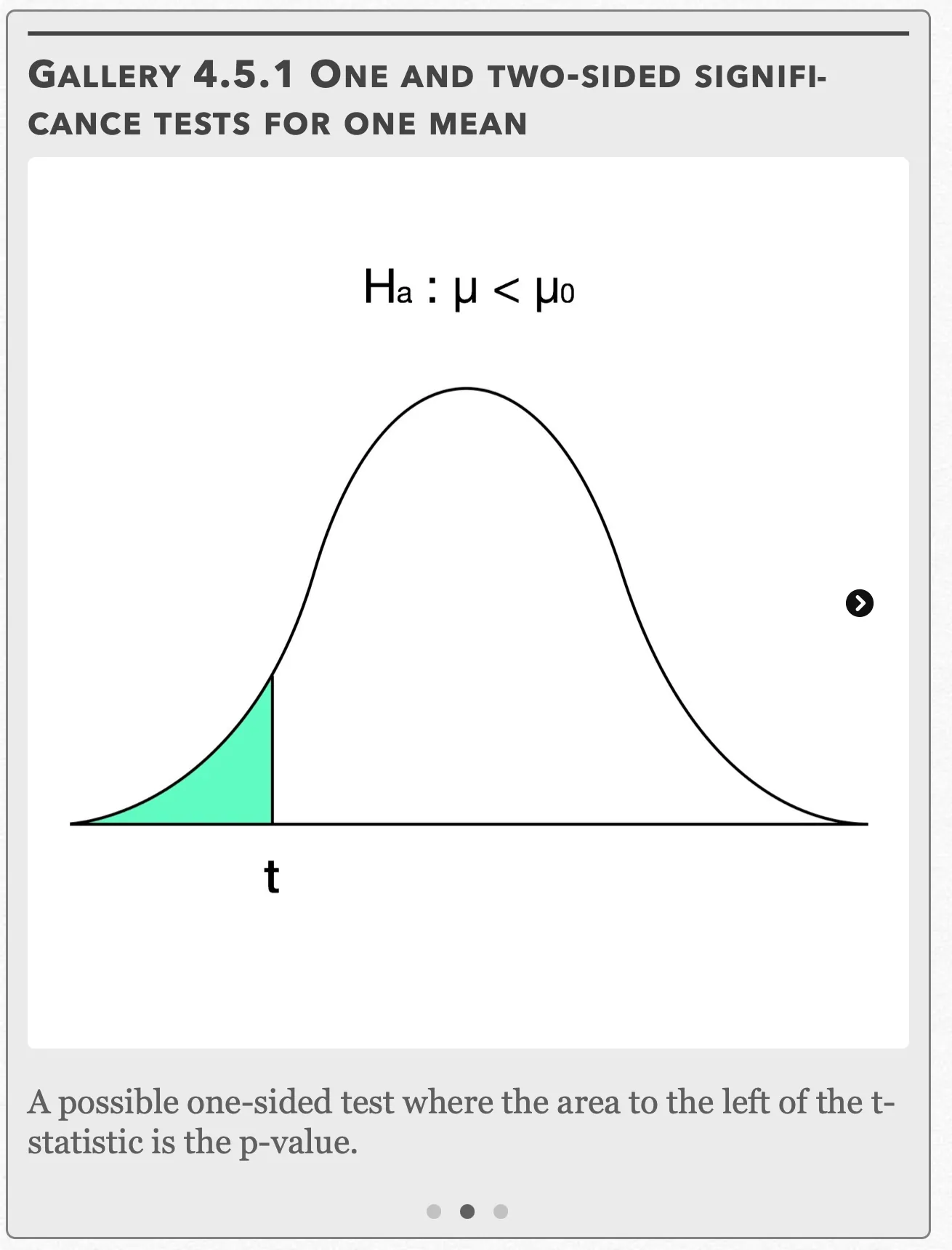
A possible one-sided test where the area to the left of the t-statistic is the p-value. Open full-size image S0410Frame 3 of 3
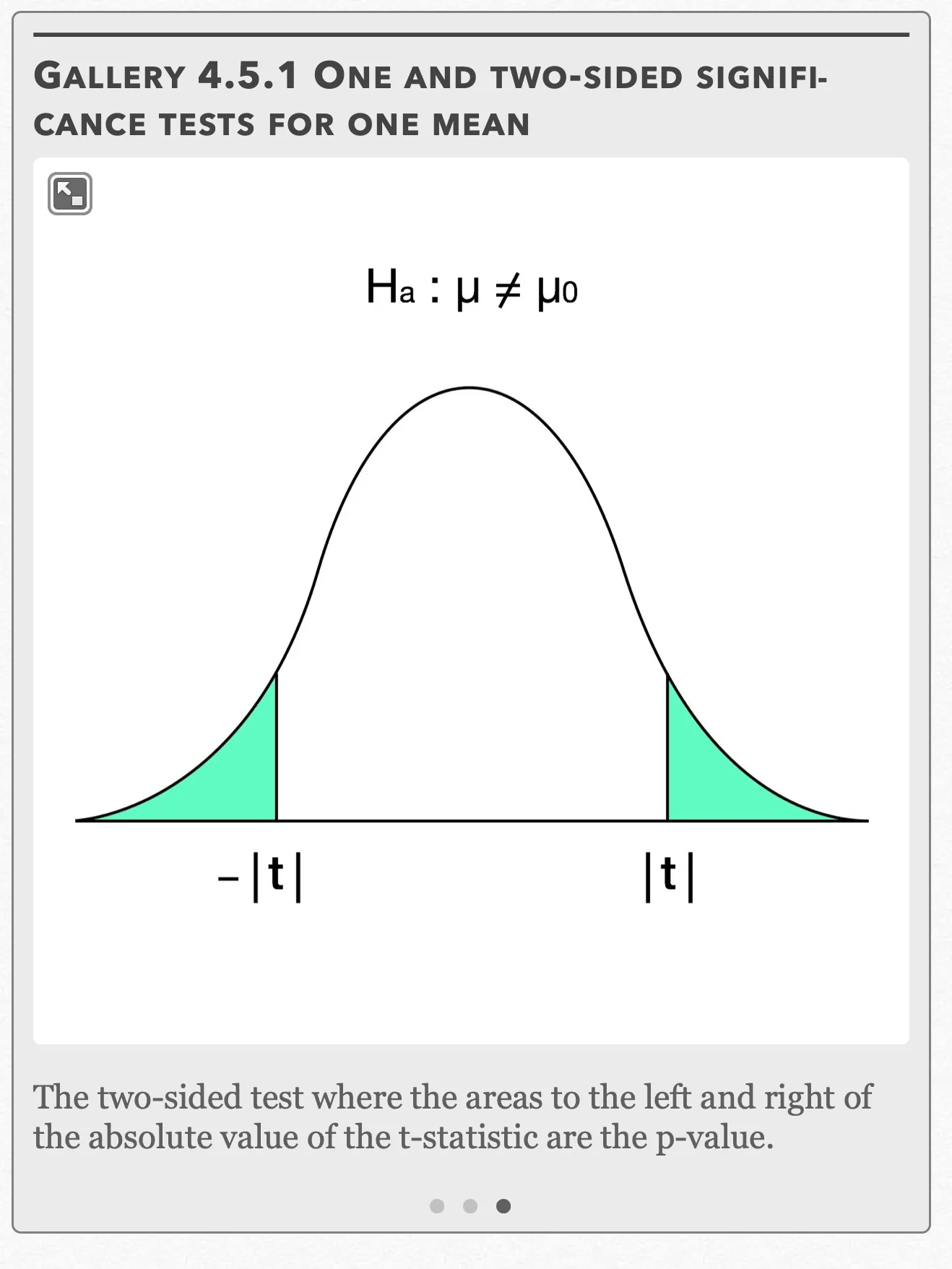
The two-sided test where the areas to the left and right of the absolute value of the t-statistic are the p-value. Open full-size image S0411
Capture provenance
Filename capture times, with no recorded timezone. Frames above follow the original gallery positions.
- · S0409 · displayed frame 1
Screenshot 2026-10-05 at 4.03.56 PM.png - · S0410 · displayed frame 2
Screenshot 2026-10-05 at 4.04.01 PM.png - · S0411 · displayed frame 3
Screenshot 2026-10-05 at 4.04.05 PM.png
Normal Condition for Small Sample Sizes
The three conditions needed for performing one-sample t-procedures can be found in Chapter 4.1. However, the Normal Condition warrants further explanation. We already know if the sample size is n ≥ 30, then the one-sample t-procedures can automatically be used due to the Central Limit TheoremEditorial qualification: The captured n ≥ 30 statement is not a universal guarantee. Under the CLT’s assumptions, the accuracy of a Normal approximation depends on the population and sample size.. This holds true even if the distribution is clearly skewed. However, does this spell “game over” if our sample size is less than 30? Not necessarily. For sample sizes n < 15, t-procedures can be used if the data appears close to Normal (no skewness or outliers). For sample sizes 15 ≤ n ≤ 30, the t-procedures can be used as long is there isn’t any strong skewness or outliers.
Gallery 4.5.2 t-table
Frame 1 of 2
This part of the t table gives the corresponding t-values from df=1 to df=18 Open full-size image S0412Frame 2 of 2
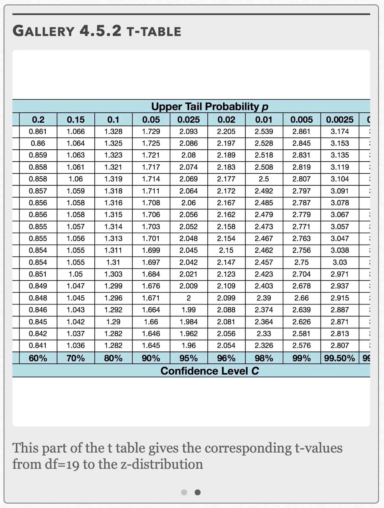
This part of the t table gives the corresponding t-values from df=19 to the z-distribution Open full-size image S0413
Capture provenance
Filename capture times, with no recorded timezone. Frames above follow the original gallery positions.
- · S0412 · displayed frame 1
Screenshot 2026-10-05 at 4.04.08 PM.png - · S0413 · displayed frame 2
Screenshot 2026-10-05 at 4.04.13 PM.png
| Captured row | p=.2 | p=.15 | p=.1 | p=.05 | p=.025 | p=.02 | p=.01 | p=.005 | p=.0025 |
|---|---|---|---|---|---|---|---|---|---|
| 1 | 1.376 | 1.963 | 3.078 | 6.314 | 12.71 | 15.89 | 31.82 | 63.66 | 127.3 |
| 2 | 1.061 | 1.386 | 1.886 | 2.92 | 4.303 | 4.849 | 6.965 | 9.925 | 14.09 |
| 3 | 0.978 | 1.25 | 1.638 | 2.353 | 3.182 | 3.482 | 4.541 | 5.841 | 7.453 |
| 4 | 0.941 | 1.19 | 1.533 | 2.132 | 2.776 | 2.999 | 3.747 | 4.604 | 5.598 |
| 5 | 0.92 | 1.156 | 1.476 | 2.015 | 2.571 | 2.757 | 3.365 | 4.032 | 4.773 |
| 6 | 0.906 | 1.134 | 1.44 | 1.943 | 2.447 | 2.612 | 3.143 | 3.707 | 4.317 |
| 7 | 0.896 | 1.119 | 1.415 | 1.895 | 2.365 | 2.517 | 2.998 | 3.499 | 4.029 |
| 8 | 0.889 | 1.108 | 1.397 | 1.86 | 2.306 | 2.449 | 2.896 | 3.355 | 3.833 |
| 9 | 0.883 | 1.1 | 1.383 | 1.833 | 2.262 | 2.398 | 2.821 | 3.25 | 3.69 |
| 10 | 0.879 | 1.093 | 1.372 | 1.812 | 2.228 | 2.359 | 2.764 | 3.169 | 3.581 |
| 11 | 0.876 | 1.088 | 1.363 | 1.796 | 2.201 | 2.328 | 2.718 | 3.106 | 3.497 |
| 12 | 0.873 | 1.083 | 1.356 | 1.782 | 2.179 | 2.303 | 2.681 | 3.055 | 3.428 |
| 13 | 0.87 | 1.079 | 1.35 | 1.771 | 2.16 | 2.282 | 2.65 | 3.012 | 3.372 |
| 14 | 0.868 | 1.076 | 1.345 | 1.761 | 2.145 | 2.264 | 2.624 | 2.977 | 3.326 |
| 15 | 0.866 | 1.074 | 1.341 | 1.753 | 2.131 | 2.249 | 2.602 | 2.947 | 3.286 |
| 16 | 0.865 | 1.071 | 1.337 | 1.746 | 2.12 | 2.235 | 2.583 | 2.921 | 3.252 |
| 17 | 0.863 | 1.069 | 1.333 | 1.74 | 2.11 | 2.224 | 2.567 | 2.898 | 3.222 |
| 18 | 0.862 | 1.067 | 1.33 | 1.734 | 2.101 | 2.214 | 2.552 | 2.878 | 3.197 |
| Captured row | p=.2 | p=.15 | p=.1 | p=.05 | p=.025 | p=.02 | p=.01 | p=.005 | p=.0025 |
|---|---|---|---|---|---|---|---|---|---|
| 1 | 0.861 | 1.066 | 1.328 | 1.729 | 2.093 | 2.205 | 2.539 | 2.861 | 3.174 |
| 2 | 0.86 | 1.064 | 1.325 | 1.725 | 2.086 | 2.197 | 2.528 | 2.845 | 3.153 |
| 3 | 0.859 | 1.063 | 1.323 | 1.721 | 2.08 | 2.189 | 2.518 | 2.831 | 3.135 |
| 4 | 0.858 | 1.061 | 1.321 | 1.717 | 2.074 | 2.183 | 2.508 | 2.819 | 3.119 |
| 5 | 0.858 | 1.06 | 1.319 | 1.714 | 2.069 | 2.177 | 2.5 | 2.807 | 3.104 |
| 6 | 0.857 | 1.059 | 1.318 | 1.711 | 2.064 | 2.172 | 2.492 | 2.797 | 3.091 |
| 7 | 0.856 | 1.058 | 1.316 | 1.708 | 2.06 | 2.167 | 2.485 | 2.787 | 3.078 |
| 8 | 0.856 | 1.058 | 1.315 | 1.706 | 2.056 | 2.162 | 2.479 | 2.779 | 3.067 |
| 9 | 0.855 | 1.057 | 1.314 | 1.703 | 2.052 | 2.158 | 2.473 | 2.771 | 3.057 |
| 10 | 0.855 | 1.056 | 1.313 | 1.701 | 2.048 | 2.154 | 2.467 | 2.763 | 3.047 |
| 11 | 0.854 | 1.055 | 1.311 | 1.699 | 2.045 | 2.15 | 2.462 | 2.756 | 3.038 |
| 12 | 0.854 | 1.055 | 1.31 | 1.697 | 2.042 | 2.147 | 2.457 | 2.75 | 3.03 |
| 13 | 0.851 | 1.05 | 1.303 | 1.684 | 2.021 | 2.123 | 2.423 | 2.704 | 2.971 |
| 14 | 0.849 | 1.047 | 1.299 | 1.676 | 2.009 | 2.109 | 2.403 | 2.678 | 2.937 |
| 15 | 0.848 | 1.045 | 1.296 | 1.671 | 2 | 2.099 | 2.39 | 2.66 | 2.915 |
| 16 | 0.846 | 1.043 | 1.292 | 1.664 | 1.99 | 2.088 | 2.374 | 2.639 | 2.887 |
| 17 | 0.845 | 1.042 | 1.29 | 1.66 | 1.984 | 2.081 | 2.364 | 2.626 | 2.871 |
| 18 | 0.842 | 1.037 | 1.282 | 1.646 | 1.962 | 2.056 | 2.33 | 2.581 | 2.813 |
| 19 | 0.841 | 1.036 | 1.282 | 1.645 | 1.96 | 2.054 | 2.326 | 2.576 | 2.807 |
Confidence Level C, in the visible column order: 60%, 70%, 80%, 90%, 95%, 96%, 98%, 99%, 99.50%.
Example 4.5.1
Recall in Chapter 1.1 that a local candy company wanted to find out how many boxes of each of their nine flavors had been sold in a week. The company now wants to create a perfume line out of its flavors. One flavor in particular, “Omnom Orange”, is said to last for 12 hours. To test this, the company takes a random sample of 16 people out of thousands from their focus group. The results are shown in the following table:
| 11.14 | 13.06 | 12.11 | 13.25 |
| 13.33 | 12.36 | 11.77 | 13.69 |
| 12.56 | 11.83 | 13.42 | 12.29 |
| 12.99 | 12.05 | 14.01 | 11.25 |
(a) Is there sufficient evidence at the α = 0.05 level to conclude that the perfume doesn’t last 12 hours?
(b) Construct a confidence interval consistent with the results in (a).
Example 4.5.1 — solution (a)
(a) First, we want to check our three conditions:
Random: The 16 people were taken from a random sample.
Normal: According to our Normal conditions for small sample sizes, for a sample size of 16, t-procedures can be used as long is there isn’t any strong skewness or outliers. To examine these conditions, we can draw graphs that enable us to easily detect skewness and outliers. We have a few choices here, but a histogram, boxplot, and/or Normal probability plot are some of the ones most commonly.
Gallery 4.5.3 Example 4.5.1 (Checking the normal condition)
Frame 1 of 8
Press the STAT button and under EDIT, select “Edit” and press ENTER Open full-size image S0414Frame 2 of 8
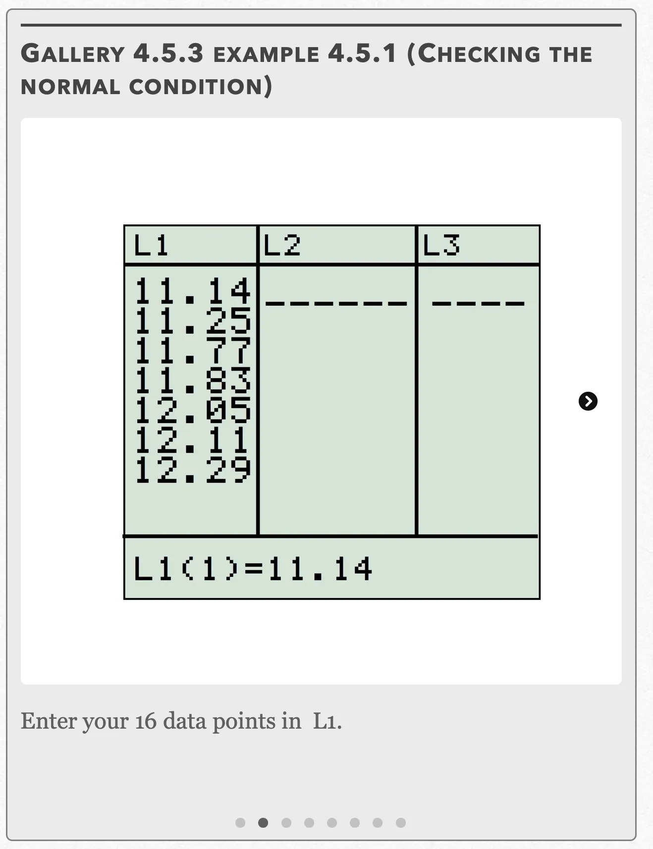
Enter your 16 data points in L1. Open full-size image S0415Frame 3 of 8
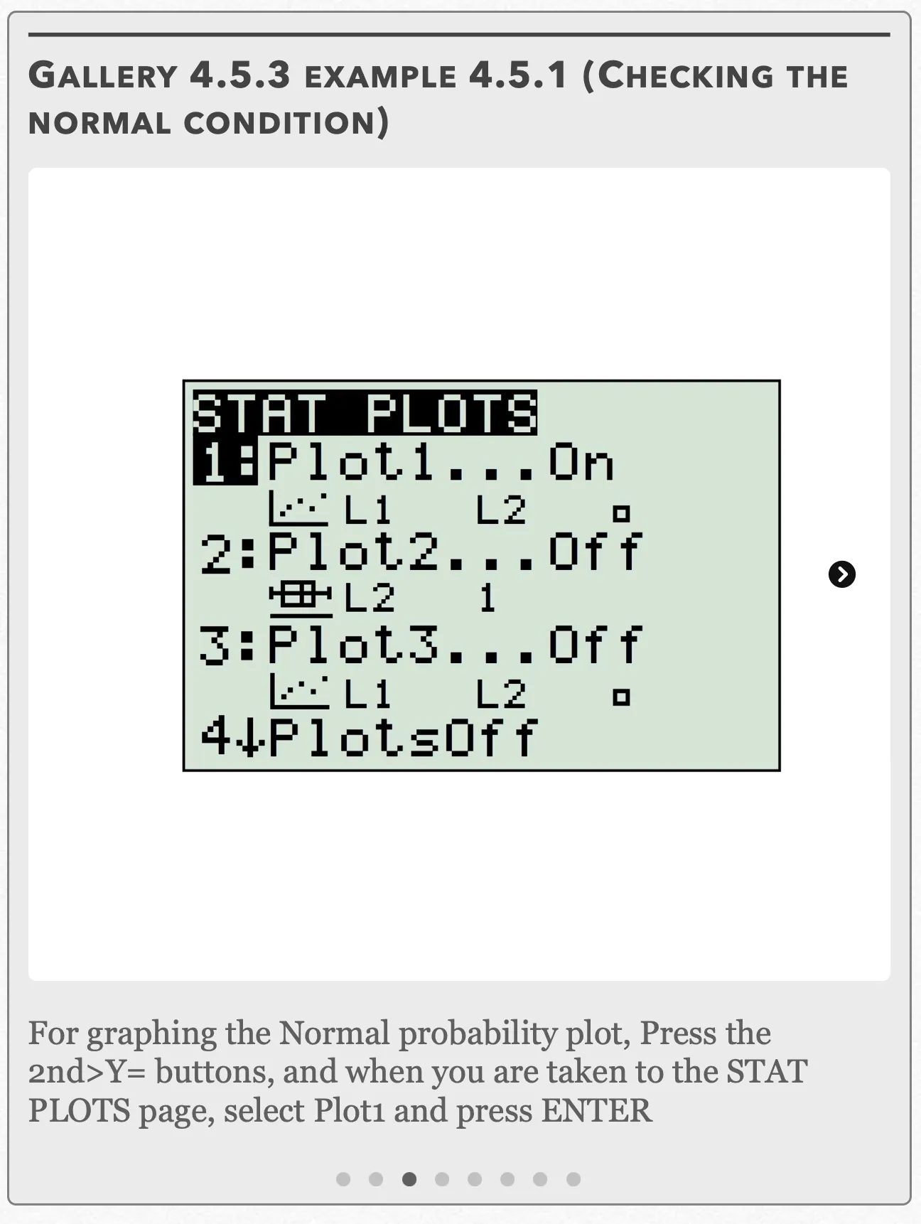
For graphing the Normal probability plot, press the 2nd>Y= buttons, and when you are taken to the STAT PLOTS page, select Plot1 and press ENTER Open full-size image S0416Frame 4 of 8
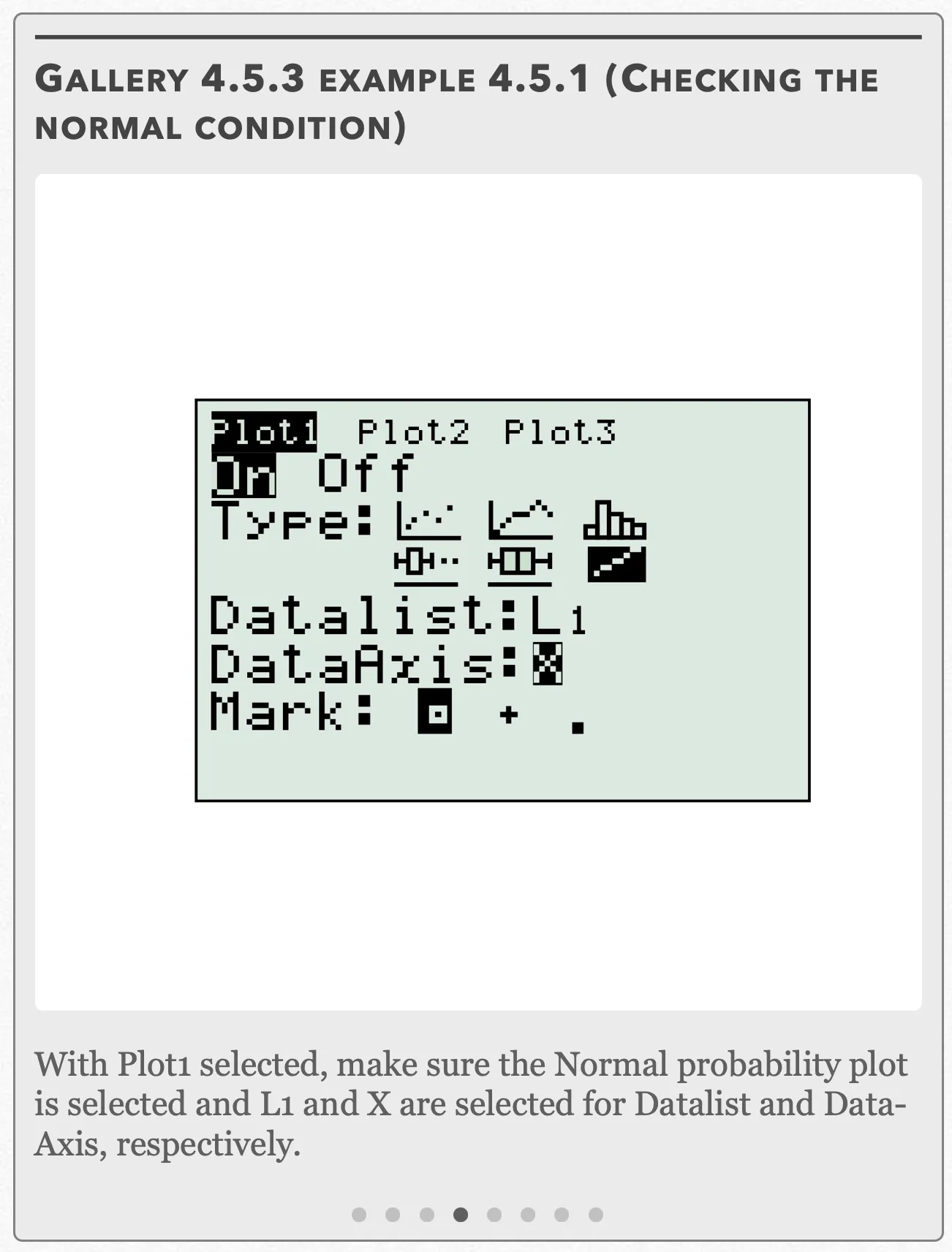
With Plot1 selected, make sure the Normal probability plot is selected and L1 and X are selected for Datalist and Data-Axis, respectively. Open full-size image S0417Frame 5 of 8
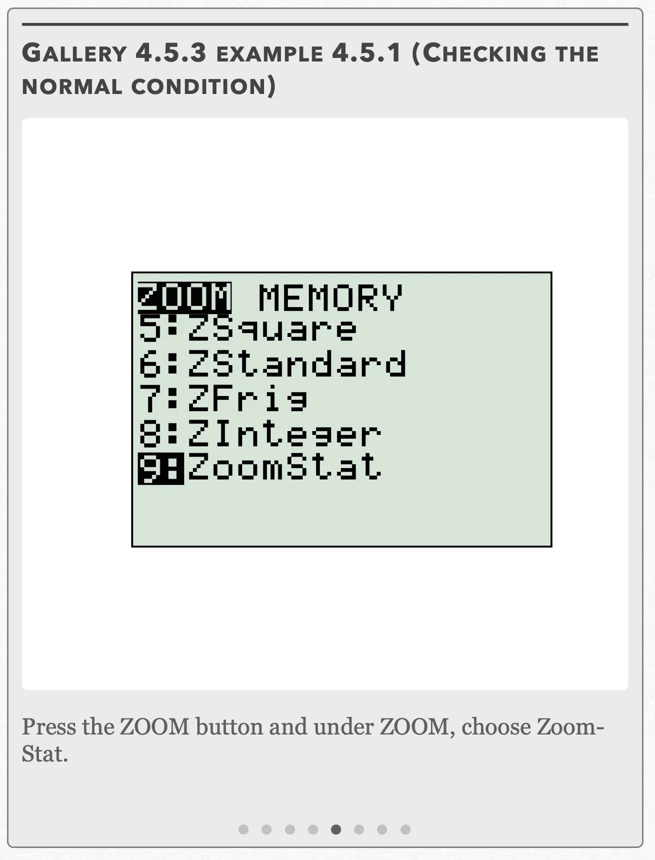
Press the ZOOM button and under ZOOM, choose ZoomStat. Open full-size image S0418Frame 6 of 8
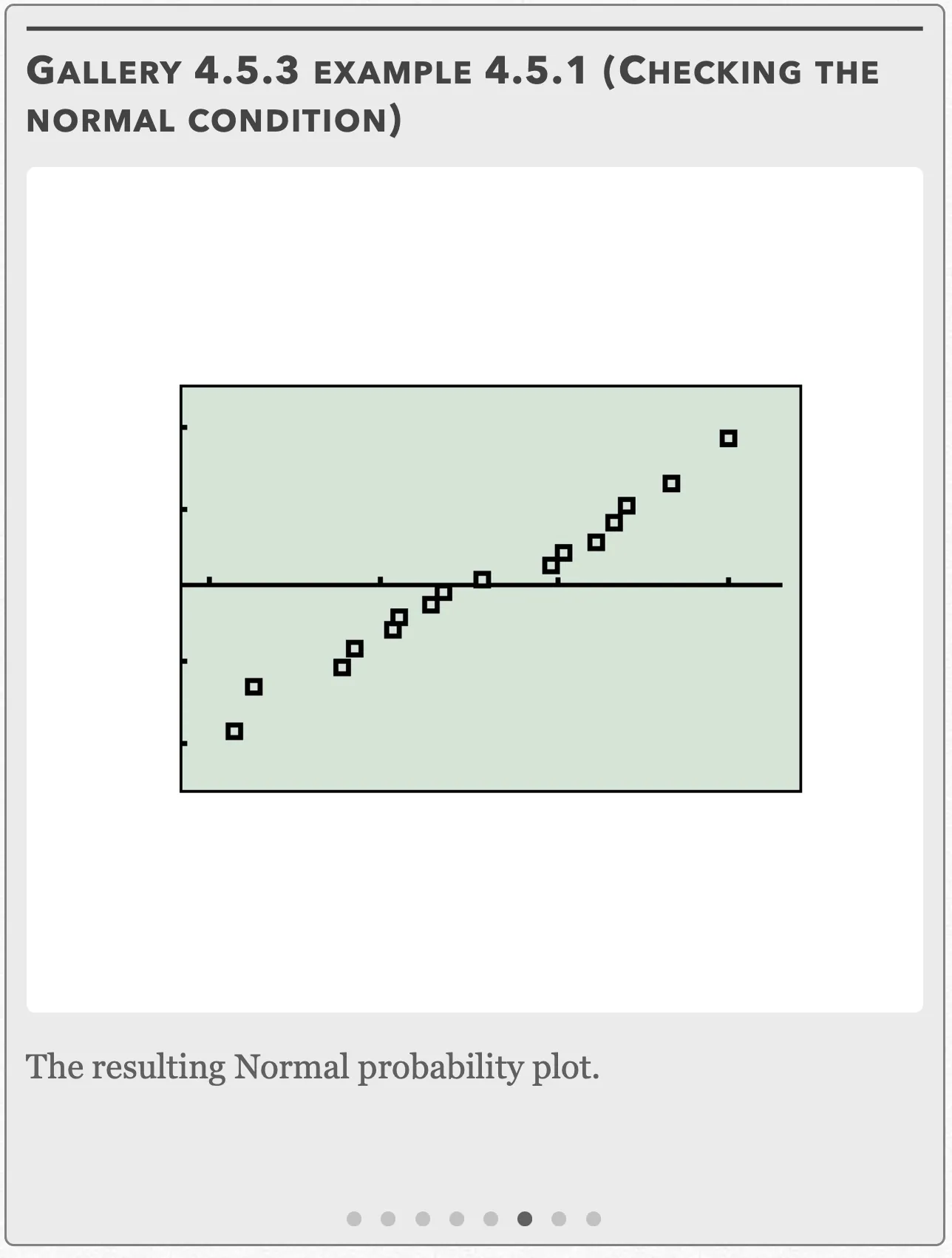
The resulting Normal probability plot. Open full-size image S0419Frame 7 of 8
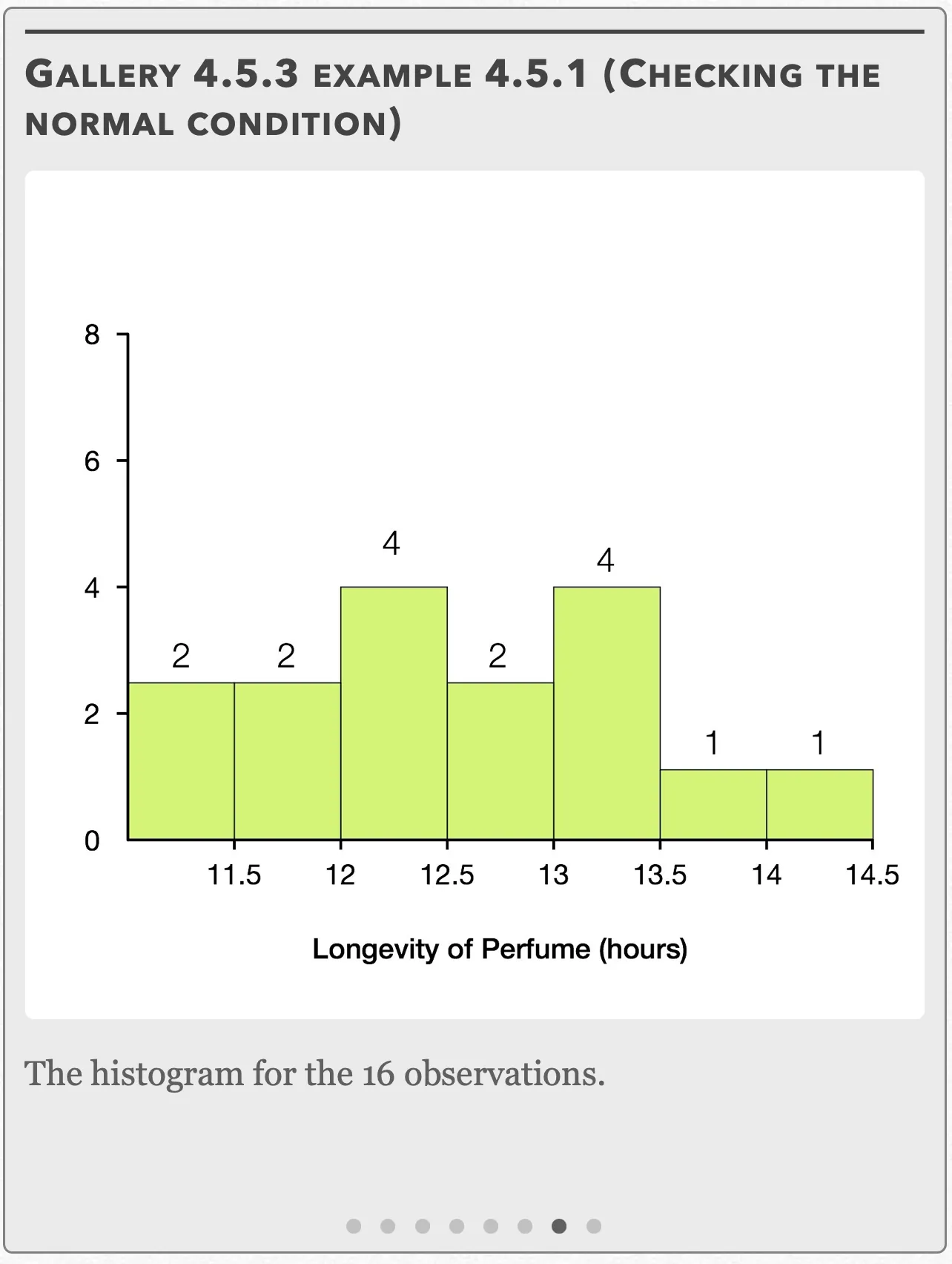
The histogram for the 16 observations. Open full-size image S0420Frame 8 of 8
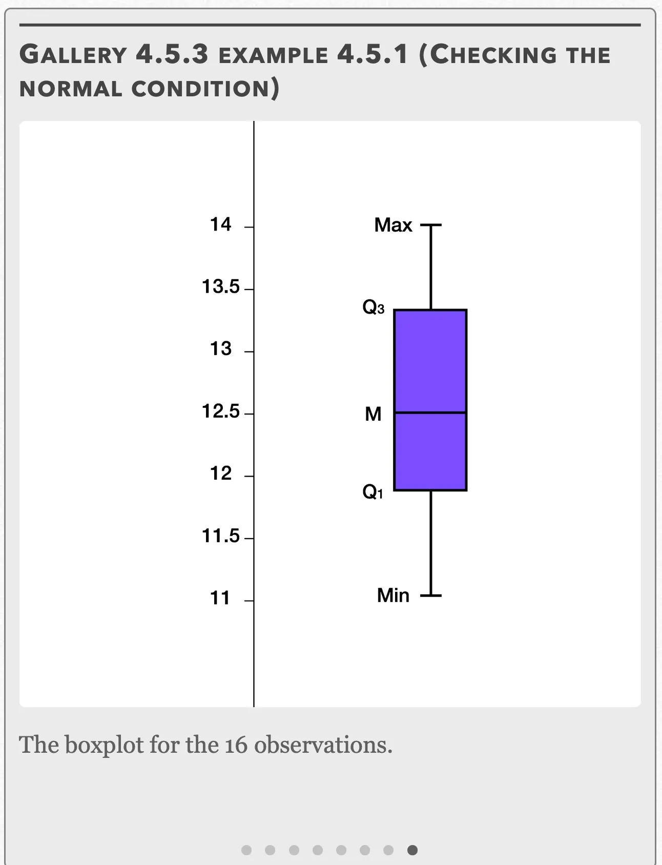
The boxplot for the 16 observations. Open full-size image S0421
Capture provenance
Filename capture times, with no recorded timezone. Frames above follow the original gallery positions.
- · S0414 · displayed frame 1
Screenshot 2026-10-05 at 4.04.16 PM.png - · S0415 · displayed frame 2
Screenshot 2026-10-05 at 4.04.20 PM.png - · S0416 · displayed frame 3
Screenshot 2026-10-05 at 4.04.24 PM.png - · S0417 · displayed frame 4
Screenshot 2026-10-05 at 4.04.28 PM.png - · S0418 · displayed frame 5
Screenshot 2026-10-05 at 4.04.32 PM.png - · S0419 · displayed frame 6
Screenshot 2026-10-05 at 4.04.36 PM.png - · S0420 · displayed frame 7
Screenshot 2026-10-05 at 4.04.40 PM.png - · S0421 · displayed frame 8
Screenshot 2026-10-05 at 4.04.44 PM.png
These can be seen in Gallery 4.5.3. The histogram is roughly symmetric with no strong skewness, the boxplot also appears to be only slightly right-skewed with no visible outliers, and the Normal probability plot is roughly linear. All three of our techniques confirm that the data has no strong skewness or outliers and thus passes the condition.
Independent: We are sampling without replacement, so the focus group has to have at least 10(16)=160 people in it, and indeed it does since it was mentioned in the problem that it contained thousands of participants.
Since we want to know if the mean number of hours is different than 12 (not specifically greater or lesser than), we use a two-sided test.
Using the formula for the one-sample t-test, we get:
Refer to Gallery 4.5.4 for how to perform these steps on your calculator for both the “Data” and “Stats” options.
We want to compare the t-statistic to the critical t-value.
Gallery 4.5.4 Example 4.5.1 (one-sample t test on TI 83/84)
Frame 1 of 4
Press the STAT button, go to TESTS, choose “T-Test” and press ENTER Open full-size image S0423Frame 2 of 4
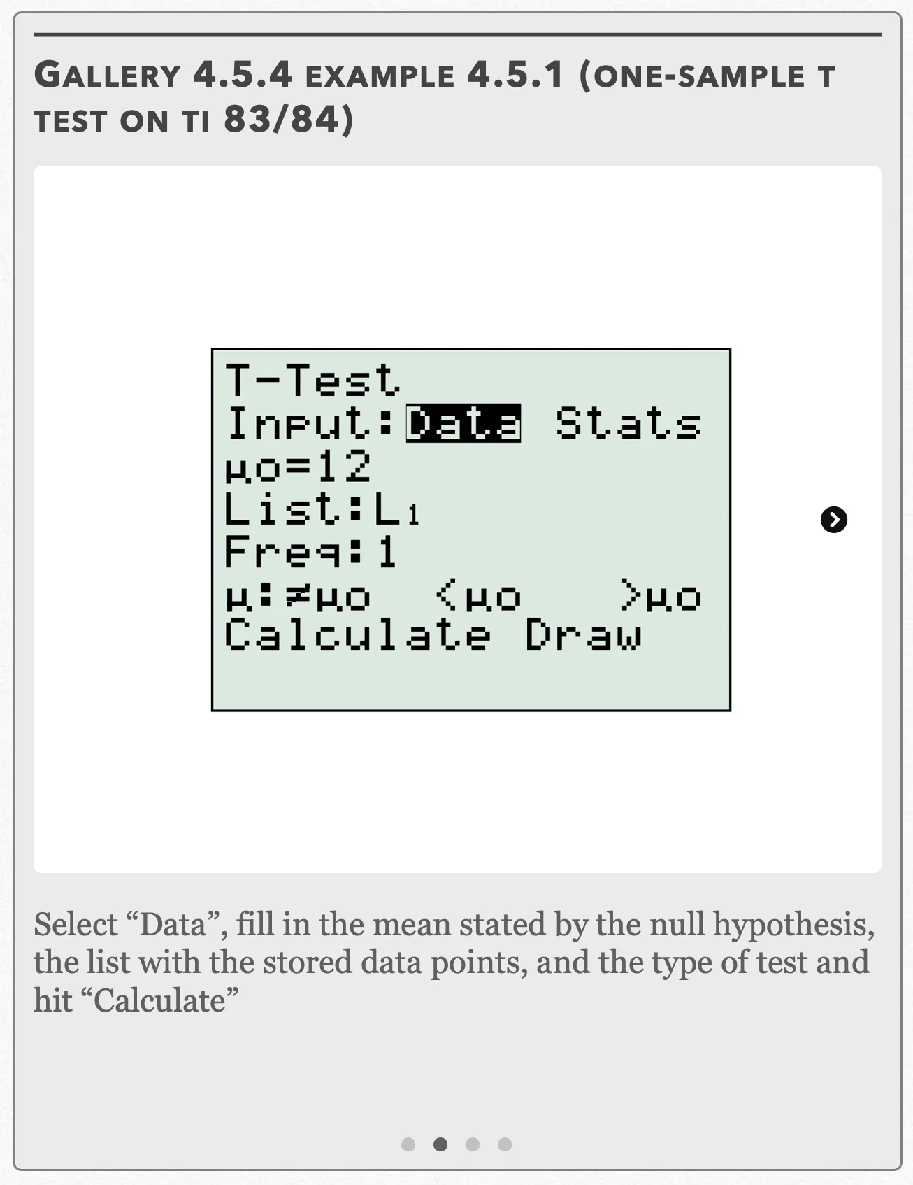
Select “Data”, fill in the mean stated by the null hypothesis, the list with the stored data points, and the type of test and hit “Calculate” Open full-size image S0424Frame 3 of 4
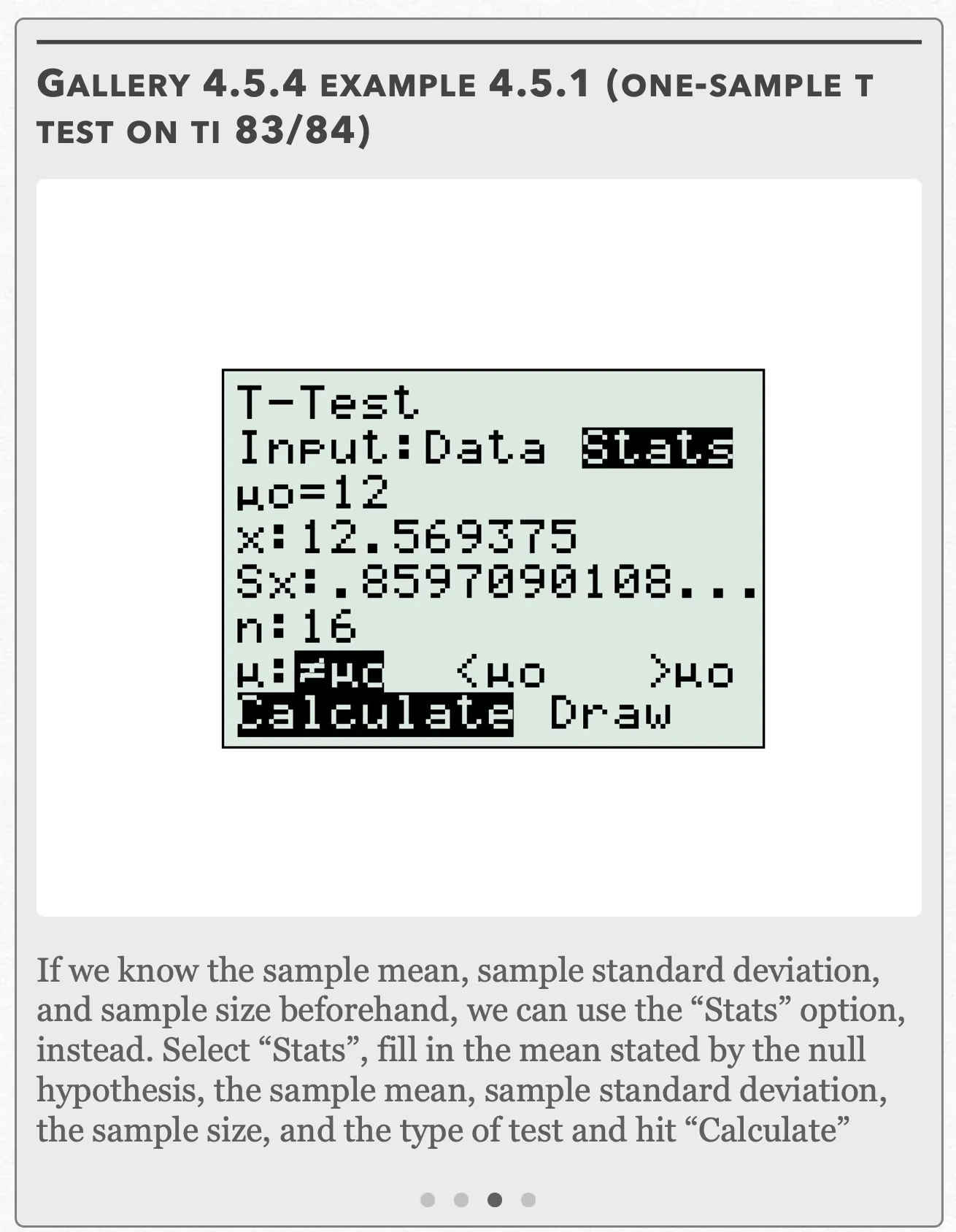
If we know the sample mean, sample standard deviation, and sample size beforehand, we can use the “Stats” option, instead. Select “Stats”, fill in the mean stated by the null hypothesis, the sample mean, sample standard deviation, the sample size, and the type of test and hit “Calculate” Open full-size image S0425Frame 4 of 4
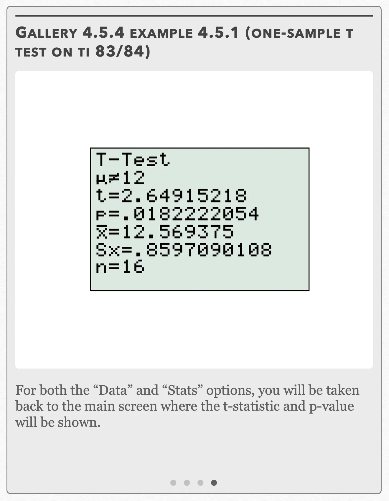
For both the “Data” and “Stats” options, you will be taken back to the main screen where the t-statistic and p-value will be shown. Open full-size image S0426
Capture provenance
Filename capture times, with no recorded timezone. Frames above follow the original gallery positions.
- · S0423 · displayed frame 1
Screenshot 2026-10-05 at 4.04.48 PM.png - · S0424 · displayed frame 2
Screenshot 2026-10-05 at 4.04.53 PM.png - · S0425 · displayed frame 3
Screenshot 2026-10-05 at 4.04.56 PM.png - · S0426 · displayed frame 4
Screenshot 2026-10-05 at 4.05.01 PM.png
To find the critical chi-square value, we need the upper tail probability and the degrees of freedom. We have a two-sided test at α = 0.05, which means the upper tail probability is 0.025 with a df = 16 − 1 = 15. With these two pieces of information, we get t* = 2.131 from the t-table.
We see that the t-statistic is greater than the critical t-value (2.649 > 2.131). Alternatively, we see that the p-value that corresponds with the t-statistic is smaller than the significance level α (0.018 < 0.05). Both results tell us that we can reject the null hypothesis and conclude that the mean number of hours the perfume lasts is different than 12.
Interactive 4.5.2 Example 4.5.1
Example 4.5.1 — solution (b)
Gallery 4.5.5 Example 4.5.1 (one-sample t interval on TI 83/84)
Frame 1 of 4
Press the STAT button, go to TESTS, choose “TInterval” and press ENTER Open full-size image S0427Frame 2 of 4
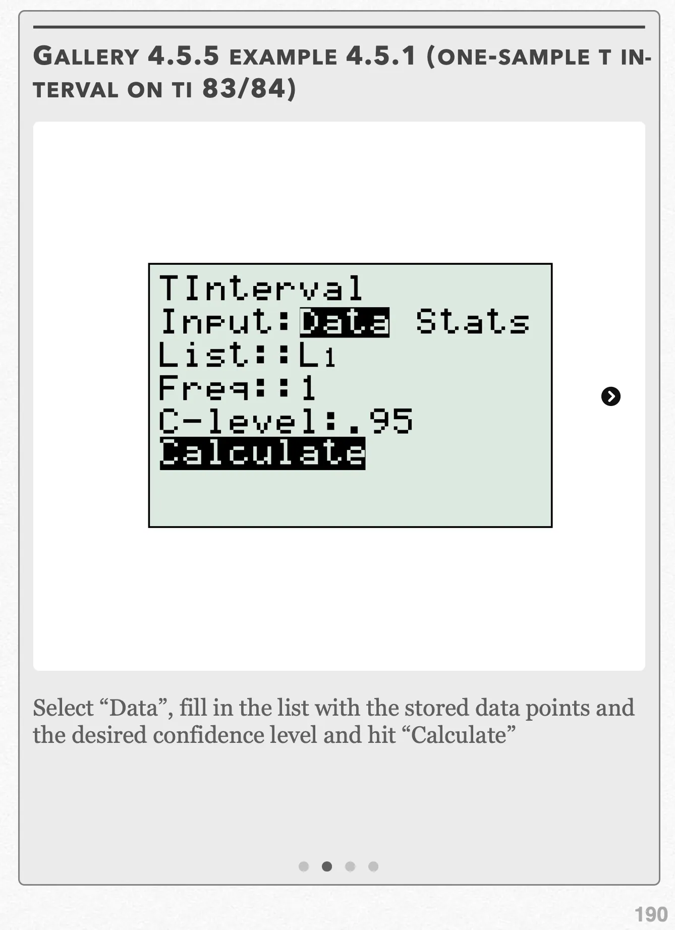
Select “Data”, fill in the list with the stored data points and the desired confidence level and hit “Calculate” Open full-size image S0428Frame 3 of 4
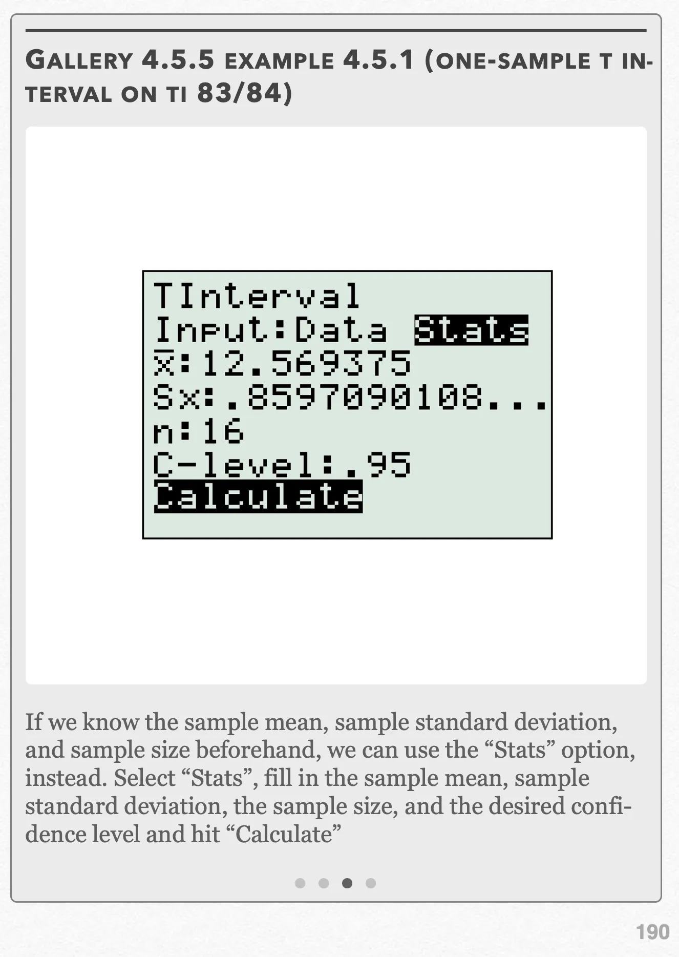
If we know the sample mean, sample standard deviation, and sample size beforehand, we can use the “Stats” option, instead. Select “Stats”, fill in the sample mean, sample standard deviation, the sample size, and the desired confidence level and hit “Calculate” Open full-size image S0429Frame 4 of 4
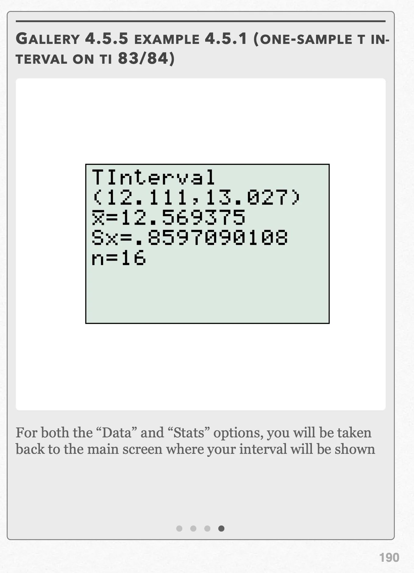
For both the “Data” and “Stats” options, you will be taken back to the main screen where your interval will be shown Open full-size image S0430
Capture provenance
Filename capture times, with no recorded timezone. Frames above follow the original gallery positions.
- · S0427 · displayed frame 1
Screenshot 2026-10-05 at 4.05.03 PM.png - · S0428 · displayed frame 2
Screenshot 2026-10-05 at 4.05.09 PM.png - · S0429 · displayed frame 3
Screenshot 2026-10-05 at 4.05.13 PM.png - · S0430 · displayed frame 4
Screenshot 2026-10-05 at 4.05.17 PM.png
(b) A confidence interval consistent with our results in (a) would have a confidence level of 95%. We already found this value to be t* = 2.131 in part (a) for 16 − 1 = 15 degrees of freedom.
Using the formula for the one-sample t-interval, we get:
Refer to Gallery 4.5.5 for how to perform these steps on your calculator.
We are 95% confident that the mean number of hours the Omnom Orange-scented perfume lasts between 12.111 and 13.027 hours. Since 12 is not included in this interval (meaning that one of the possible values the mean could take isn’t 12), this agrees with the results from the significance test in (a) where we had evidence that the perfume didn’t last 12 hours.
Pop Quiz 4.5.1
Glossary and deeper reading · 16 refreshers
These editorial refreshers supplement the reading. Definitions and examples are added guidance; original source wording and recorded answers remain in their original context.
-
T-table
A t-table lists critical values for t-distributions at specified degrees of freedom and tail probabilities. Its column convention must be checked before using it for a one-sided test or a two-sided interval. For example, a two-sided 95% interval leaves 2.5% in each tail when selecting its critical value.
-
Sample statistic
A statistic is a numerical summary calculated from sample data. Its value can change when a different sample is selected from the same population. For example, the proportion of walkers among 60 sampled students is a statistic.
Read more: Sample statistic in the captured Statistics reading →
-
Test statistic
A test statistic summarizes how the sample departs from the null model. Its reference distribution under the null supplies the probabilities used in testing. For example, a z-statistic expresses a sample proportion’s difference from a hypothesized proportion in null-model standard-error units.
Read more: Test statistic in the captured Statistics reading →
-
Standard deviation
Standard deviation measures spread around the mean using squared deviations and a square root. A sample standard deviation uses the sum of squared deviations divided by one less than the sample size before taking the square root. For example, a larger standard deviation of travel times indicates greater variability, in the original time units.
Read more: Standard deviation in the captured Statistics reading →
-
Population
A population is the full set of individuals or measurements a study aims to describe. It must be defined clearly before deciding whether a sample supports generalization. For example, all students enrolled in a particular school this year form a population.
-
Mean
The mean is a measure of center often called an average. For a finite data set, the arithmetic mean is the sum of the values divided by their number; for a random variable, the mean is its probability-weighted expected value when that value exists. Means can be pulled toward extreme values and are not generally resistant. For example, the arithmetic mean of 2, 4, and 9 is 5.
-
Null hypothesis
A null hypothesis specifies the reference claim or model used to calculate a test’s probabilities. It commonly states no population difference or a particular parameter value. For example, a null hypothesis can state that the population mean travel time equals 15 minutes.
Read more: Null hypothesis in the captured Statistics reading →
-
Sample
A sample is the subset of a population actually studied. How it is selected matters for the conclusions that can be drawn about the population. For example, 60 selected students may be a sample from a school’s full enrollment.
-
Alternative hypothesis
An alternative hypothesis specifies the population difference or direction for which a test seeks evidence. It should be chosen from the research question before inspecting results. For example, an alternative can state that the population mean travel time is greater than 15 minutes.
Read more: Alternative hypothesis in the captured Statistics reading →
-
Confidence interval
A confidence interval is a data-based range produced by a method with a specified long-run coverage rate for a population parameter. For a fixed population, the calculated interval either contains the parameter or it does not; the confidence level describes the method over repeated samples. For example, a 95% method captures the true parameter in about 95% of repeated intervals when its assumptions hold.
Read more: Confidence interval in the captured Statistics reading →
-
Simple random sample
A simple random sample of a fixed size gives every possible subset of that size the same chance of selection. Giving individuals equal selection chances alone does not establish that the design is an SRS. For example, randomly choosing three identifiers without replacement from ten gives an SRS when every three-identifier set is equally likely.
Read more: Simple random sample in the captured Statistics reading →
-
Critical value
A critical value is a cutoff from a reference distribution chosen for a confidence level or testing rule. The relevant distribution, degrees of freedom, and one-sided or two-sided procedure determine the cutoff. For example, a symmetric 95% Normal interval uses a cutoff near 1.96 standard-error units.
Read more: Critical value in the captured Statistics reading →
-
Degrees of freedom
Degrees of freedom describe the independent information remaining after constraints or estimated quantities are accounted for. The value depends on the procedure, rather than always being the sample size minus 1. For example, a one-sample t procedure uses n − 1 degrees of freedom, while simple regression inference uses n − 2.
-
Central limit theorem
Editorial qualification: The captured n ≥ 30 statement is not a universal guarantee. Under the CLT’s assumptions, the accuracy of a Normal approximation depends on the population and sample size.
For independent identically distributed observations with finite variance, the central limit theorem explains why the standardized sample mean approaches a Normal distribution as sample size increases. There is no universal sample size that makes every population sufficiently close to Normal; skewness and extreme tails affect the approximation. For example, averaging many independent waiting times can produce a less skewed distribution of averages than the original waiting-time distribution.
Read more: Central limit theorem in the captured Statistics reading →
-
Skewness
Skewness describes asymmetry in a quantitative distribution’s tails. A longer right tail indicates right skew, while a longer left tail indicates left skew. For example, many short waits with a few very long waits produce right skew.
-
Confidence level
A confidence level is the long-run fraction of intervals from a procedure that capture the true parameter under its assumptions. Holding the data and procedure fixed, increasing the confidence level generally widens the interval. For example, a 99% interval is usually wider than a 90% interval calculated from the same sample.
Read more: Confidence level in the captured Statistics reading →