4.1 Sampling Distributions for Sample Means
The Population SD Is Not the Mean’s SD
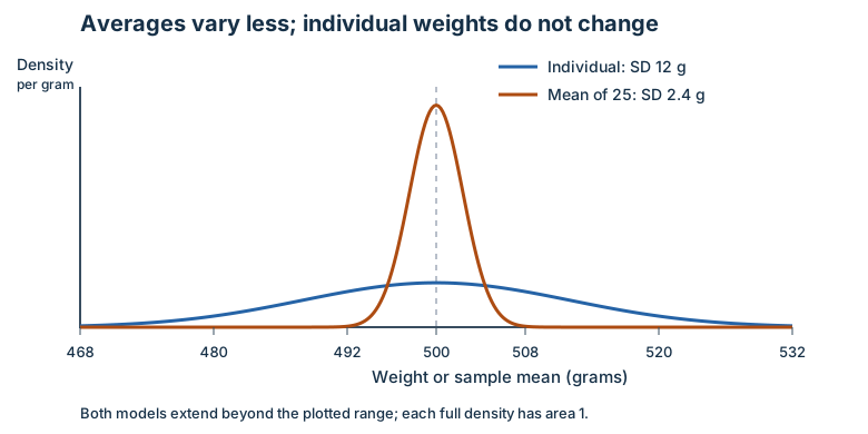
A filling process produces independently generated package weights modeled by a normal distribution with known population mean 500 grams and population SD 12 grams. Select 25 independent fills and average their weights. Some packages are above 500 and some below; averaging reduces the variability of the statistic without changing the individual-weight distribution.
For independent sampled values from a population with mean and SD ,
Here the sample-mean distribution has mean 500 grams and SD grams. Dividing by n instead of its square root would make the spread too small. The population SD remains 12 grams; only the statistic’s sampling SD becomes 2.4 grams.
Start with How the Observations Were Obtained
For a random sample without replacement from a finite population, check both random selection and , where N is the population size and n is the sample size. This small sampling fraction supports the usual approximation to independence and the SD formula without a finite-population correction. For example, an SRS of 40 from 8,000 records passes because . Forty conveniently selected records do not meet the randomization condition merely because the fraction is small.
The filling example instead explicitly supplies independently generated observations. We do not invent a finite N for that process or apply a without-replacement check where there is no without-replacement selection.
Normal Populations and the CLT Give Different Reasons
For a quantitative variable with a normal population model, the sampling distribution of the mean is normal regardless of sample size, provided the sampling assumptions hold. Thus the normal filling model allows n = 25; “less than 30” is not a reason to reject it.
If the population is not normal, the central limit theoremEditorial qualification: The captured n ≥ 30 statement is not a universal guarantee. Under the CLT’s assumptions, the accuracy of a Normal approximation depends on the population and sample size. can justify an approximately normal distribution for the mean. The course’s usual starting check is , together with the sampling conditions. The shape of the population still matters. If it is extremely skewed, a sample much larger than 30 may be needed; crossing 30 does not erase severe skew or influential extremes. Independent sampling and finite population variance underlie the CLT argument.
| Population and design | Shape conclusion for the sample mean |
|---|---|
| Normal model, 9 independent observations | Normal, even though n is below 30 |
| Moderately skewed, SRS of 40 with a small sampling fraction | An approximately normal mean model is reasonable |
| Extremely skewed, SRS of 30 | Do not justify normality from the threshold alone; a much larger sample may be needed |
| Any population, 100 volunteers instead of a random sample | The assumed random-sampling model is unsupported |
Increasing n changes the sampling distribution of the mean; collecting more simulation repetitions at the same n only gives a better view of that fixed distribution. Neither change turns the original individual values into a normal population.
Worked Example: A High Average Fill Weight
Under the supplied normal independent-fill model, the chance that the average of 25 fills exceeds 504 grams is
The mean 500 grams is the long-run average of size-25 sample means. The SD 2.4 grams is their typical deviation from that center. About 4.8% of repeated sets of 25 independent fills would have a mean above 504 grams under the model. The event concerns an average of 25, not a single heavy package; using 12 in the z denominator would answer a different question.
The values 500 and 12 were supplied as known population parameters. If one pilot sample instead reports and , those are observed statistics. They do not establish new known values of and . Estimating an unknown mean and its uncertainty belongs to inference; keep that task separate from the theoretical sampling-distribution calculation here.
Try It Yourself
The following original practice applies the ideas above to a fresh setting. Show the reasoning requested in each part. Answers and task-specific rubrics are on the separate solutions page.
Original generated practice for the Fall 2026 course.
Glossary and deeper reading · 12 refreshers
These editorial refreshers supplement the reading. Definitions and examples are added guidance; original source wording and recorded answers remain in their original context.
-
Normal distribution
A Normal distribution is a continuous, symmetric bell-shaped distribution determined by its mean and standard deviation. Many symmetric distributions are not Normal, so symmetry by itself is insufficient. For example, a Normal model centered at 50 with standard deviation 5 places most values relatively close to 50.
Read more: Normal distribution in the captured Statistics reading →
-
Mean
The mean is a measure of center often called an average. For a finite data set, the arithmetic mean is the sum of the values divided by their number; for a random variable, the mean is its probability-weighted expected value when that value exists. Means can be pulled toward extreme values and are not generally resistant. For example, the arithmetic mean of 2, 4, and 9 is 5.
-
Population
A population is the full set of individuals or measurements a study aims to describe. It must be defined clearly before deciding whether a sample supports generalization. For example, all students enrolled in a particular school this year form a population.
-
Sample
A sample is the subset of a population actually studied. How it is selected matters for the conclusions that can be drawn about the population. For example, 60 selected students may be a sample from a school’s full enrollment.
-
Sample statistic
A statistic is a numerical summary calculated from sample data. Its value can change when a different sample is selected from the same population. For example, the proportion of walkers among 60 sampled students is a statistic.
Read more: Sample statistic in the captured Statistics reading →
-
Random sampling
Random sampling uses a specified chance process to select individuals from a population. It supports population inference when the sampling frame and data collection are appropriate, but does not guarantee perfect balance or eliminate every source of bias. For example, a random-number generator can select student identifiers from an enrollment list.
Read more: Random sampling in the captured Statistics reading →
-
Sampling without replacement
Sampling without replacement does not return selected items before later selections. Selections from a finite population are dependent, although treating them as approximately independent can be reasonable when the sample is a small fraction of the population. For example, selecting students without replacement ensures that no student is chosen twice.
Read more: Sampling without replacement in the captured Statistics reading →
-
Quantitative variable
A quantitative variable records a numerical count or measurement for each individual. Differences between its values have a meaningful numerical interpretation. For example, the number of books borrowed and the mass of a backpack are quantitative variables.
Read more: Quantitative variable in the captured Statistics reading →
-
Sampling distribution
A sampling distribution describes how a statistic varies across all possible samples drawn under a specified sampling design and sample size. It is a distribution of statistics rather than of individual observations. For example, the proportions from repeated random samples of 60 students form a sampling distribution.
Read more: Sampling distribution in the captured Statistics reading →
-
Central limit theorem
Editorial qualification: The captured n ≥ 30 statement is not a universal guarantee. Under the CLT’s assumptions, the accuracy of a Normal approximation depends on the population and sample size.
For independent identically distributed observations with finite variance, the central limit theorem explains why the standardized sample mean approaches a Normal distribution as sample size increases. There is no universal sample size that makes every population sufficiently close to Normal; skewness and extreme tails affect the approximation. For example, averaging many independent waiting times can produce a less skewed distribution of averages than the original waiting-time distribution.
Read more: Central limit theorem in the captured Statistics reading →
-
Statistical independence
Statistical independence means that learning one outcome does not change the probability distribution of another. For two events, it implies that the probability of both occurring equals the product of their probabilities. For example, independent draws with replacement keep the second draw’s color probabilities unchanged by the first.
Read more: Statistical independence in the captured Statistics reading →
-
Simulation
A simulation imitates a chance process using a specified model. Repeated simulated outcomes can approximate probabilities when the model faithfully represents the situation. For example, random digits can model repeated draws from a bag with known color proportions.