4.7 Intervals and Tests for Regression Lines
Section Overview
- Interactive 4.7.1 — Inference w/ LSR lines
- Gallery 4.7.1 — 1 & 2 sided tests for LSR line
- Example 4.7.1
- Gallery 4.7.2 — Checking for Conditions
- Gallery 4.7.3 — t-test for slope on Calc
- Pop Quiz 4.7.1
Using Sample Regression Lines
Back when we first introduced and used regression lines in Chapter 1.5, we were actually referring to sample regression lines, regression lines that relied on sample data. We create and analyze sample regression lines in order to estimate the true or population regression line.
There are five conditions that must be met before inference procedures can be carried out on the sample regression line:
Random — The data we use comes from a random sample or randomized experiment.
Normal — For fixed x-values, the response y is Normally distributed. This concept is illustrated in Interactive 4.7.1. We can check for Normality by making a stemplot, Normal probability plot, or histogram from the residuals to check for any strong skewness, outliers, or other apparent departures from Normality. Since we are using t-procedures, similar rules apply to the sample size to when we were performing them for the sample mean.
Independent — Individual observations are independent of one another. If we are sampling without replacement we want to make sure that the population is at least 10 times as large as the sample, or .
Linear — The relationship between x and y is actually linear. For fixed x-values, the mean response μᵧ falls on the population regression line , where α and β are the unknown population parameters of sample intercept a and sample slope b, respectively. We can check for this condition by checking the scatterplot for a roughly linear pattern and making a residual plot to see if points are randomly scattered about the residual line.
Interactive 4.7.1 Inference with least-square regression lines
Equal Variance — For all values of x, the standard deviation of y is the same, where the standard deviation proper σ is an unknown population parameter. To check this condition, make a residual plot and check that there is a fairly equal amount of scatter about the residual line.
Significance Tests for Regression Lines
When performing significance tests for the sample regression line, we use the t test for the slope to find the t-statistic for linear regression:
where b = sample slope; β₀ = population slope stated by null hypothesis; SEᵦ = standard error of the slope.
Our null hypothesis is: .
We also have our three possible alternative hypotheses, where:
See Gallery 4.7.1 for a visualization of one and two-sided tests.
Confidence Intervals for Regression Lines
The t interval for the slope is:
where b = sample slope; t* = critical t-value; SEᵦ = standard error of the slope.
Gallery 4.7.1 One and two-sided significance tests for regression line
Frame 1 of 3
A possible one-sided test where the area to the right of the t-statistic for the slope is the p-value. Open full-size image S0459Frame 2 of 3
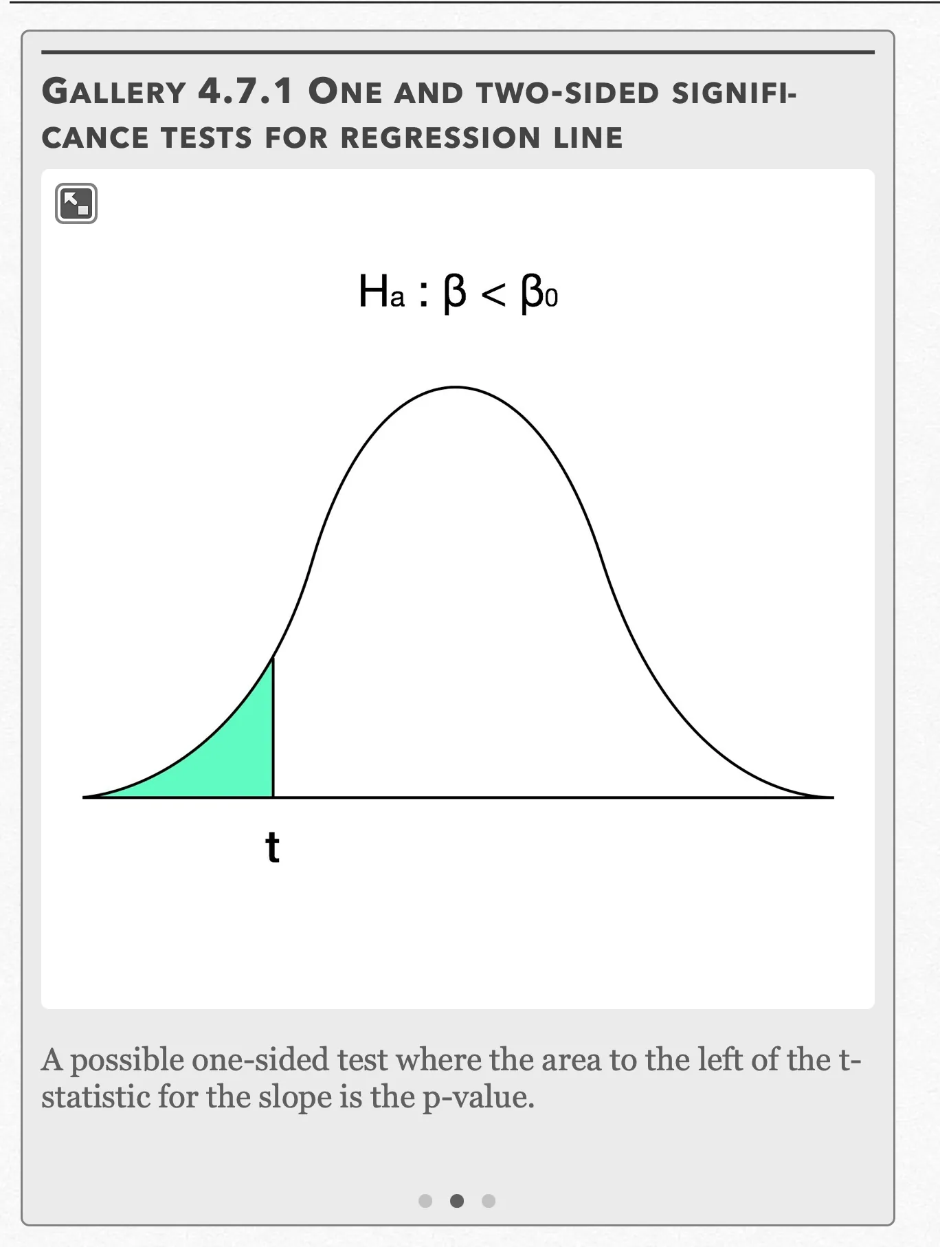
A possible one-sided test where the area to the left of the t-statistic for the slope is the p-value. Open full-size image S0460Frame 3 of 3
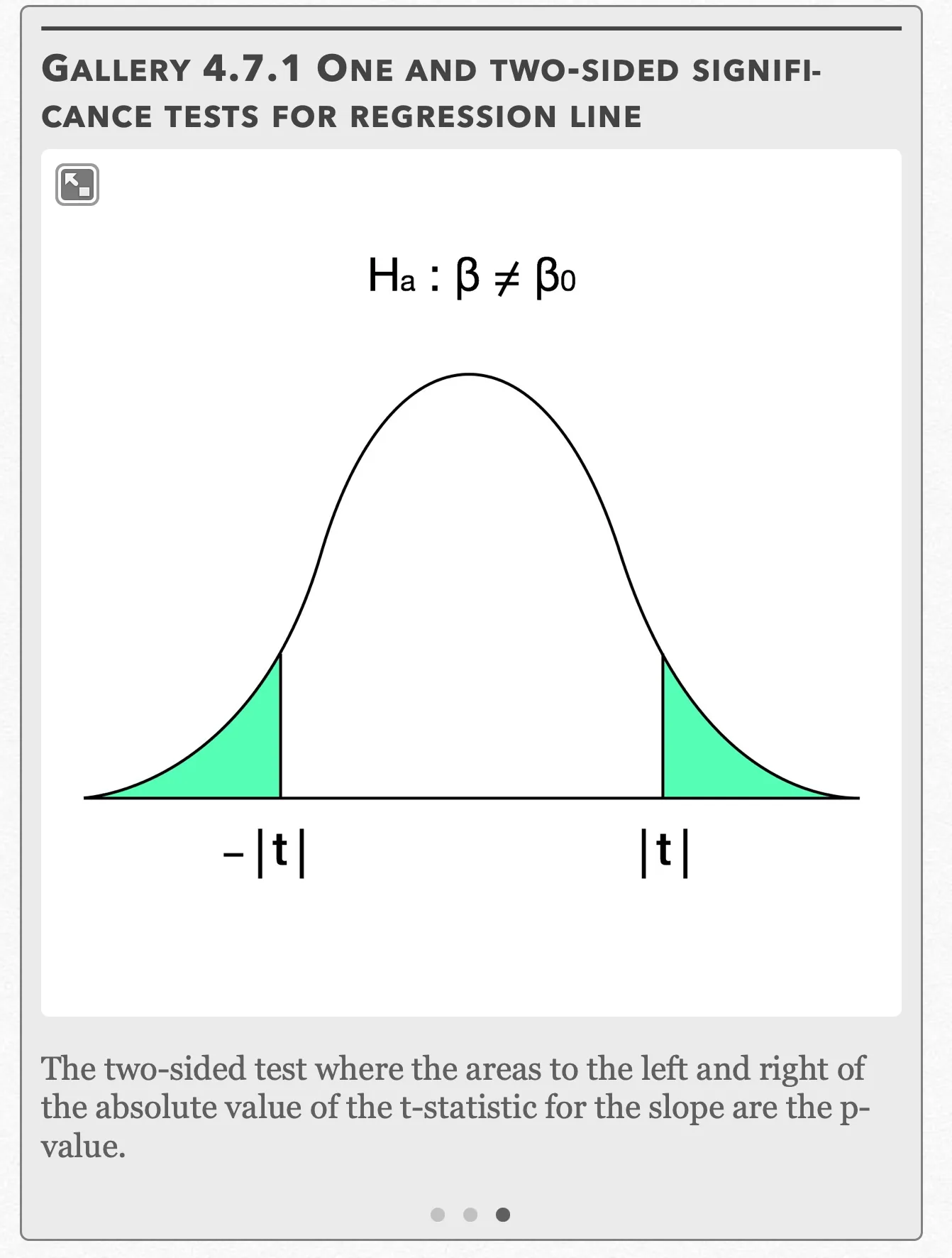
The two-sided test where the areas to the left and right of the absolute value of the t-statistic for the slope are the p-value. Open full-size image S0461
Capture provenance
Filename capture times, with no recorded timezone. Frames above follow the original gallery positions.
- · S0459 · displayed frame 1
Screenshot 2026-10-05 at 4.06.24 PM.png - · S0460 · displayed frame 2
Screenshot 2026-10-05 at 4.06.29 PM.png - · S0461 · displayed frame 3
Screenshot 2026-10-05 at 4.06.33 PM.png
Example 4.7.1
Hundreds of people compete in Granular Glory, a sand castle-building contest held every year. After watching a few rounds, you suspect that there is a (positive) relationship between the size of the sand castle sculpture and the score received from the judges. To test this, you take a random sample of 19 contestants and record the volume of their sculpture and the score they received from the judges, where the maximum score is 150. The results are shown in the following table:
| Sandcastle Volume (m³) | Contest Score |
|---|---|
| 11.76 | 67 |
| 12.37 | 88 |
| 12.89 | 81 |
| 13.67 | 77 |
| 13.72 | 84 |
| 14.02 | 82 |
| 14.53 | 93 |
| 15.11 | 105 |
| 15.62 | 92 |
| 15.43 | 94 |
| 16.09 | 84 |
| 16.37 | 104 |
| 17.30 | 112 |
| 17.49 | 123 |
| 18.32 | 111 |
| 18.73 | 118 |
| 19.55 | 127 |
| 20.96 | 136 |
| 22.42 | 129 |
(a) Is there sufficient evidence at the α = 0.05 level to conclude that there is a relationship between sand castle volume and contest score?
(b) Construct a confidence interval consistent with the results in (a).
Example 4.7.1 — solution (a)
Gallery 4.7.2 Example 4.7.1 (Checking various conditions)
Frame 1 of 6
L1 and L2 contain the x and observed y values from the example, while L3 contains the predicted y-values from the regression line. Open full-size image S0462Frame 2 of 6
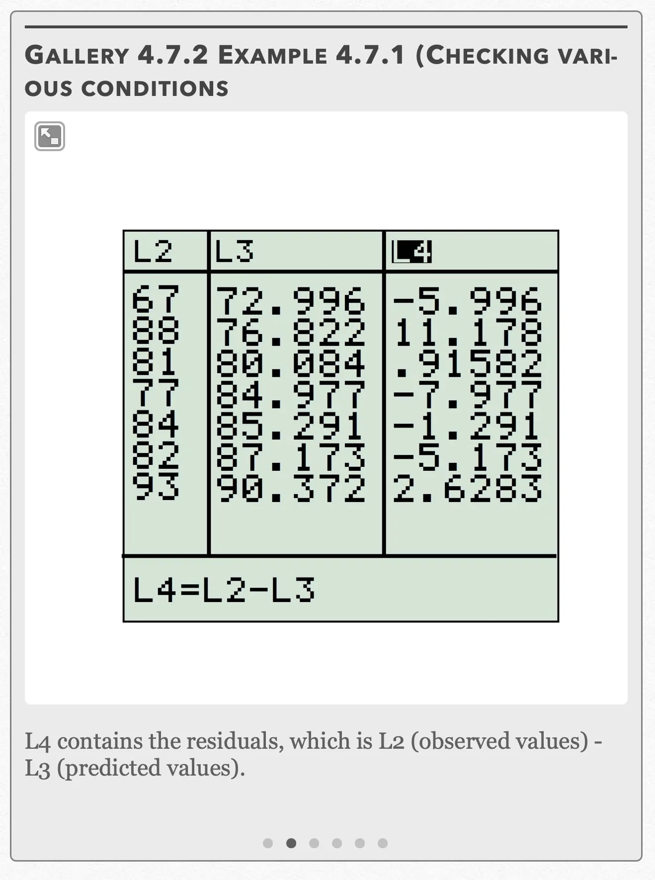
L4 contains the residuals, which is L2 (observed values) - L3 (predicted values). Open full-size image S0463Frame 3 of 6
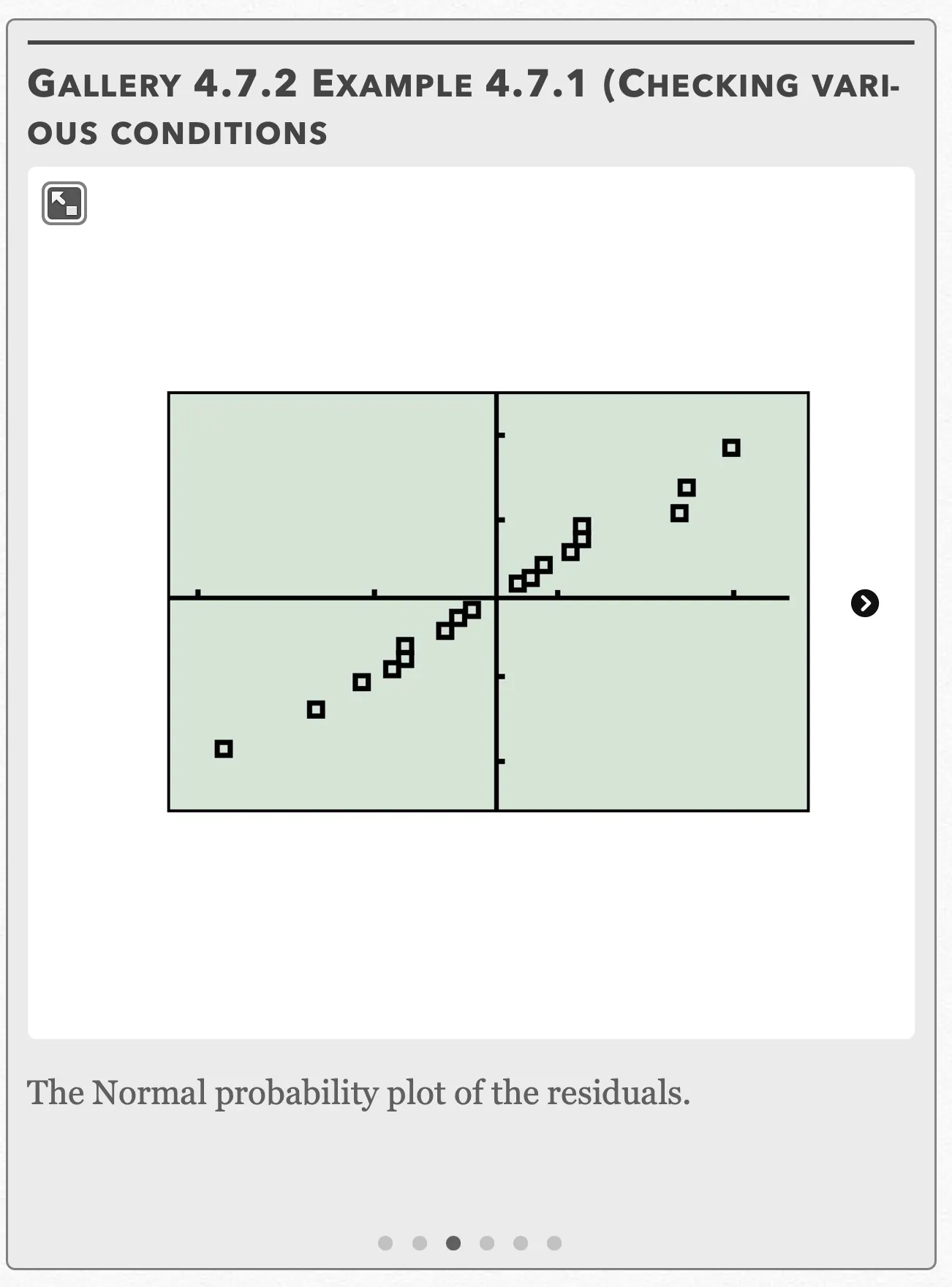
The Normal probability plot of the residuals. Open full-size image S0464Frame 4 of 6
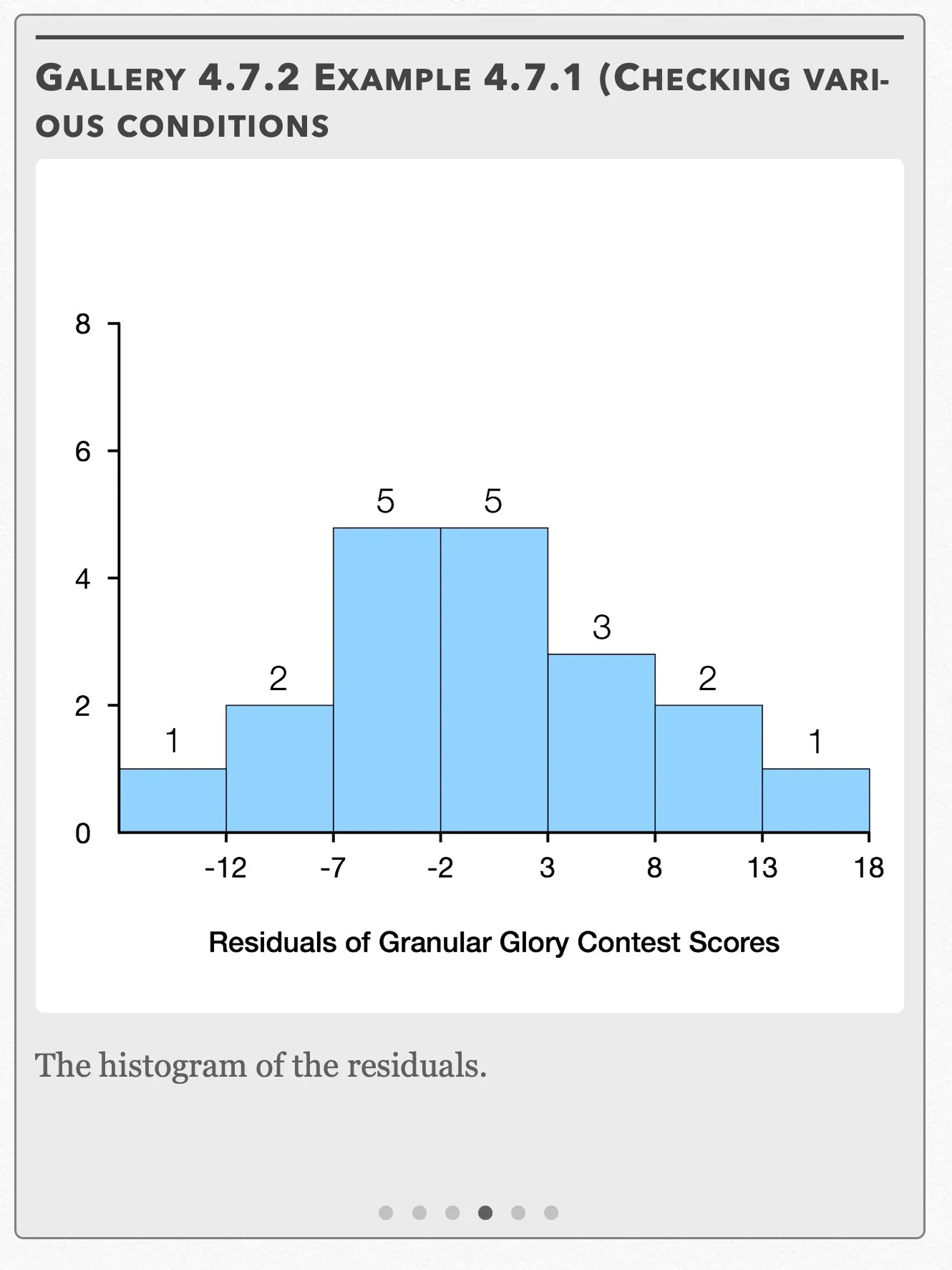
The histogram of the residuals. Open full-size image S0465Frame 5 of 6
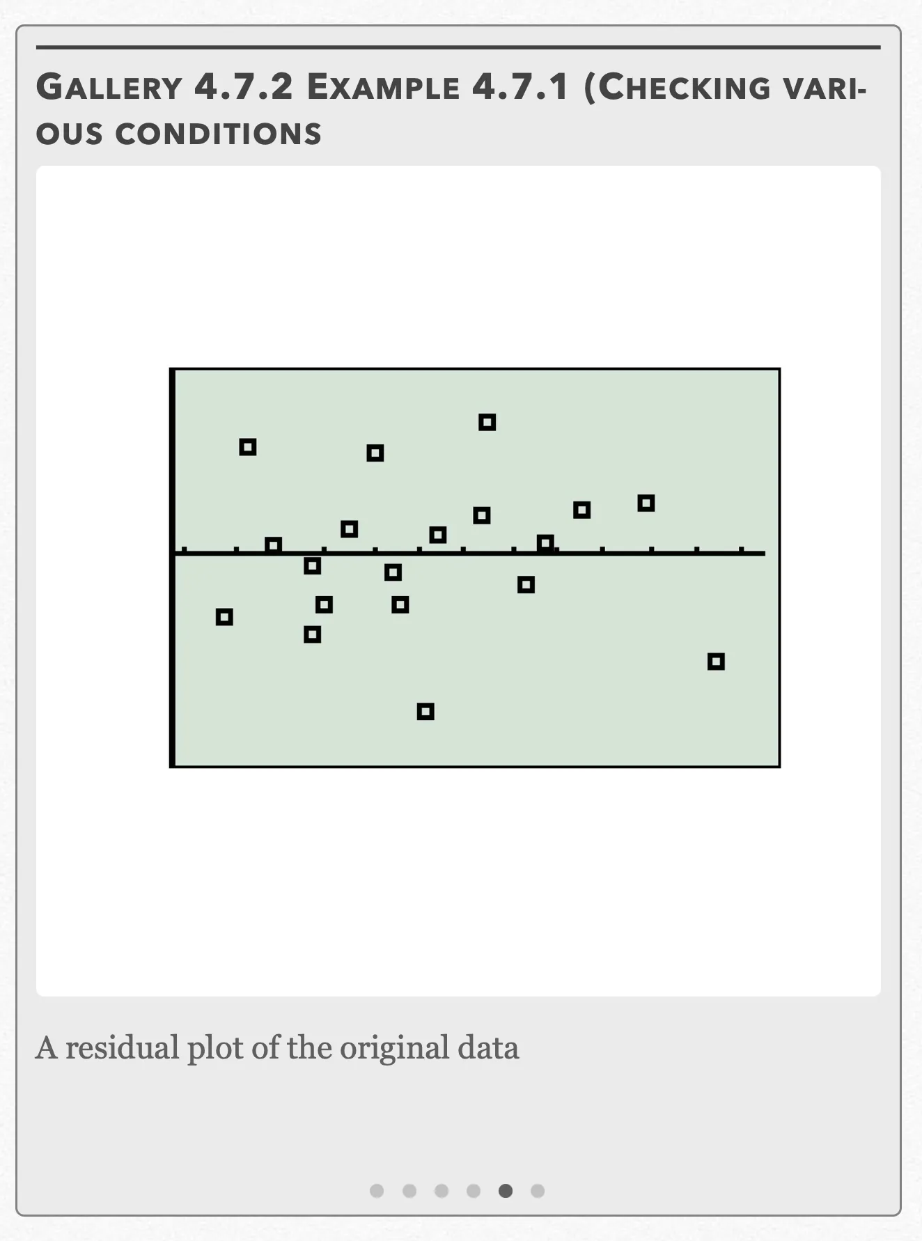
A residual plot of the original data Open full-size image S0466Frame 6 of 6
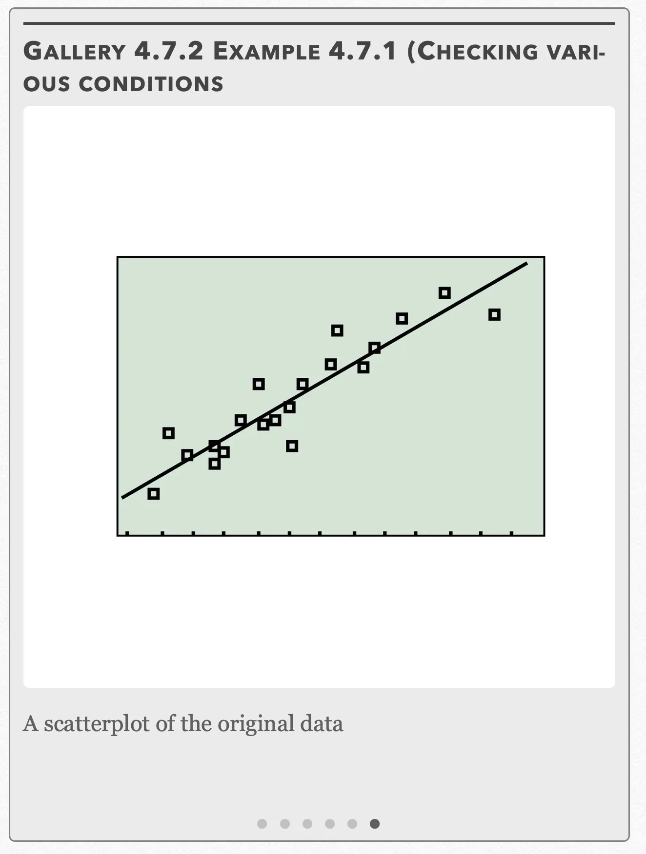
A scatterplot of the original data Open full-size image S0467
Capture provenance
Filename capture times, with no recorded timezone. Frames above follow the original gallery positions.
- · S0462 · displayed frame 1
Screenshot 2026-10-05 at 4.06.36 PM.png - · S0463 · displayed frame 2
Screenshot 2026-10-05 at 4.06.40 PM.png - · S0464 · displayed frame 3
Screenshot 2026-10-05 at 4.06.43 PM.png - · S0465 · displayed frame 4
Screenshot 2026-10-05 at 4.06.47 PM.png - · S0466 · displayed frame 5
Screenshot 2026-10-05 at 4.06.51 PM.png - · S0467 · displayed frame 6
Screenshot 2026-10-05 at 4.06.55 PM.png
The calculator lists visible in the first two gallery frames are:
| L1 (x) | L2 (observed y) | L3 (predicted y) | L4 (residual) |
|---|---|---|---|
| 11.76 | 67 | 72.996 | −5.996 |
| 12.37 | 88 | 76.822 | 11.178 |
| 12.89 | 81 | 80.084 | .91582 |
| 13.67 | 77 | 84.977 | −7.977 |
| 13.72 | 84 | 85.291 | −1.291 |
| 14.02 | 82 | 87.173 | −5.173 |
| 14.53 | 93 | 90.372 | 2.6283 |
(a) First, we want to check our five conditions:
Random: The 19 contestants were taken from a random sample.
Normal: Gallery 4.7.2 shows a histogram and a Normal probability plot of the residuals (see Gallery 4.5.3 for a full explanation of creating a Normal Probability Plot on your calculator.) The histogram is roughly symmetrical with no strong skewness. The Normal probability plot is roughly linear. These two techniques confirm that the data follows a roughly Normal distribution and thus passes the condition.
Independent: We are sampling without replacement, so the population has to have at least 10(19)=190 people in it, which is not an unreasonable assumption since it was stated in the problem that hundreds of people compete in Granular Glory every year.
Linear: Looking at the scatterplot of the data in Gallery 4.7.2, we see it takes a roughly linear pattern (see Gallery 1.5.2 for a full explanation of creating a scatterplot on your calculator.) Additionally when we look at the residual plot in Gallery 4.7.2, we see that the points are randomly scattered about the residual line. (See Gallery 1.6.1 for a full explanation of creating a residual plot on your calculator.)
Equal Variance: Looking at the residual plot again, we see that there is a fairly equal amount of scatter about the residual line.
Since we want to know if there is a positive association between sand castle volume and contest score, we use the one-sided test where:
Using the t test for the slope to calculate the t-statistic for regression, we get:
However, since there is no easy way to find SEᵦ on the calculator, we cannot compute the test statistic manually. Luckily, we can use the LinRegTTest function on our calculator to get the job done. Refer to Gallery 4.7.3 for the steps.
Gallery 4.7.3 Example 4.7.1 (t-test for the slope on TI 83/84)
Frame 1 of 3
Press the STAT button, go to TESTS, choose “LinRegTTest” and press ENTER Open full-size image S0469Frame 2 of 3
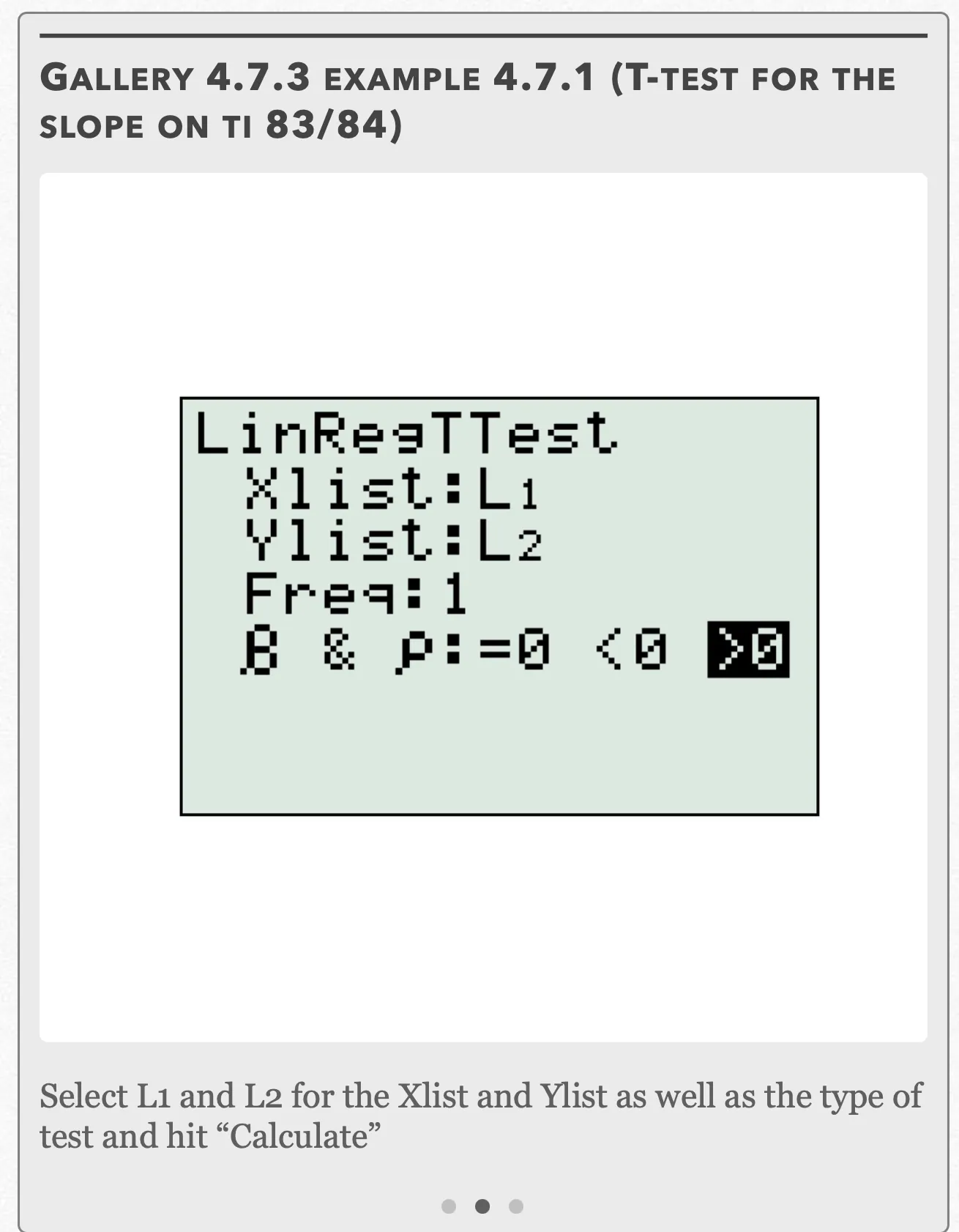
Select L1 and L2 for the Xlist and Ylist as well as the type of test and hit “Calculate” Open full-size image S0470Frame 3 of 3
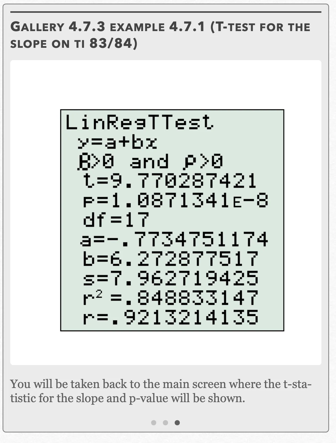
You will be taken back to the main screen where the t-statistic for the slope and p-value will be shown. Open full-size image S0471
Capture provenance
Filename capture times, with no recorded timezone. Frames above follow the original gallery positions.
- · S0469 · displayed frame 1
Screenshot 2026-10-05 at 4.06.59 PM.png - · S0470 · displayed frame 2
Screenshot 2026-10-05 at 4.07.03 PM.png - · S0471 · displayed frame 3
Screenshot 2026-10-05 at 4.07.06 PM.png
After completing the test we get a t-statistic for regression of t = 9.770 which corresponds to a p-value of 1.087 · 10⁻⁸.
Since , we can reject the null hypothesis and conclude that there is a (positive) relationship between the size of a contestant’s castle and the score received from the judges.
Example 4.7.1 — solution (b)
(b) Since confidence intervals are inherently two-sided and our significance test was one-sided, we want to use a confidence level at 90%. To find the critical t-value t*, we need to refer to the t-table. The critical t-value at 90% and degrees of freedom df = 19 − 2 = 17 is t* = 1.740. Assuming the x and y values are still stored in L₁ and L₂, performing the LinReg(a+bx) function in the calculator, should yield b = 6.2729 for the sample slope (Refer to Gallery 1.5.3 for more details.) Finally, the standard error of the slope can be derived from rearranging the test statistic equation from the t test for the slope:
Using the formula for the t-interval for the slope, we get:
We are 90% confident that for every increase in sand castle size by 1 m³, there is an increase in score between 5.156 points and 7.390 points. Since 0 is not included in this interval (meaning that the score has to increase when the castle size increases), this agrees with the results from the significance test in (a) where we rejected the null hypothesis of β = 0.
Pop Quiz 4.7.1
Glossary and deeper reading · 16 refreshers
These editorial refreshers supplement the reading. Definitions and examples are added guidance; original source wording and recorded answers remain in their original context.
-
Least-squares regression
Least-squares regression fits a line predicting a response from an explanatory variable. The fitted line minimizes the sum of squared vertical residuals between observed and predicted responses. For example, a fitted line can predict a plant’s height from its age, within the range of observed ages.
Read more: Least-squares regression in the captured Statistics reading →
-
Sample
A sample is the subset of a population actually studied. How it is selected matters for the conclusions that can be drawn about the population. For example, 60 selected students may be a sample from a school’s full enrollment.
-
Random sampling
Random sampling uses a specified chance process to select individuals from a population. It supports population inference when the sampling frame and data collection are appropriate, but does not guarantee perfect balance or eliminate every source of bias. For example, a random-number generator can select student identifiers from an enrollment list.
Read more: Random sampling in the captured Statistics reading →
-
Experiment
An experiment deliberately imposes treatments and measures responses. Random assignment, comparison, and replication help distinguish treatment effects from other variation. For example, assigning plants to fertilizer treatments is an experiment.
-
Stemplot
A stemplot splits each numerical observation into a stem and a leaf. A key specifies the place values, so the original observations can be recovered. For example, a key of 3 | 7 = 37 means that stem 3 with leaf 7 represents 37.
-
Normal probability plot
A Normal probability plot compares ordered observations with the pattern expected from a Normal distribution. A roughly straight pattern supports the approximation, while strong curvature or isolated points can reveal departures. For example, a residual Normal probability plot can help assess a regression model’s Normal-error assumption.
-
Statistical independence
Statistical independence means that learning one outcome does not change the probability distribution of another. For two events, it implies that the probability of both occurring equals the product of their probabilities. For example, independent draws with replacement keep the second draw’s color probabilities unchanged by the first.
Read more: Statistical independence in the captured Statistics reading →
-
Observation
An observation is a recorded value or set of values for an individual or occasion. The individual may be a person, object, or event rather than a human subject. For example, one plant’s measured height is an observation in a plant-growth study.
-
Mean
The mean is a measure of center often called an average. For a finite data set, the arithmetic mean is the sum of the values divided by their number; for a random variable, the mean is its probability-weighted expected value when that value exists. Means can be pulled toward extreme values and are not generally resistant. For example, the arithmetic mean of 2, 4, and 9 is 5.
-
Population
A population is the full set of individuals or measurements a study aims to describe. It must be defined clearly before deciding whether a sample supports generalization. For example, all students enrolled in a particular school this year form a population.
-
Significance test
A significance test assesses how compatible observed data are with a specified null model. It compares a test statistic or p-value with a decision rule chosen for the study. For example, a test can assess whether a sample provides evidence that a population walking proportion differs from a stated value.
Read more: Significance test in the captured Statistics reading →
-
Regression slope
A regression slope is the predicted change in the response for a one-unit increase in the explanatory variable. Its units are response units per explanatory-variable unit. For example, a slope of 2 centimeters per week predicts 2 additional centimeters of height for each additional week.
Read more: Regression slope in the captured Statistics reading →
-
Null hypothesis
A null hypothesis specifies the reference claim or model used to calculate a test’s probabilities. It commonly states no population difference or a particular parameter value. For example, a null hypothesis can state that the population mean travel time equals 15 minutes.
Read more: Null hypothesis in the captured Statistics reading →
-
Alternative hypothesis
An alternative hypothesis specifies the population difference or direction for which a test seeks evidence. It should be chosen from the research question before inspecting results. For example, an alternative can state that the population mean travel time is greater than 15 minutes.
Read more: Alternative hypothesis in the captured Statistics reading →
-
Critical value
A critical value is a cutoff from a reference distribution chosen for a confidence level or testing rule. The relevant distribution, degrees of freedom, and one-sided or two-sided procedure determine the cutoff. For example, a symmetric 95% Normal interval uses a cutoff near 1.96 standard-error units.
Read more: Critical value in the captured Statistics reading →
-
Standard error
A standard error describes the standard deviation of a statistic’s sampling distribution, usually estimated from data. It measures uncertainty in an estimate rather than the spread of individual observations. For example, the estimated standard error of a sample mean is the sample standard deviation divided by the square root of the sample size.
Read more: Standard error in the captured Statistics reading →