4.8 Chi Square Tests
Section Overview
- Interactive 4.8.1 — Chi-square Curves
- Gallery 4.8.1 — Chi-square Table
- Example 4.8.1
- Gallery 4.8.2 — 1-Way Chi-sq. Test on Calc
- Interactive 4.8.2 — Example 4.8.1
- Example 4.8.2
- Gallery 4.8.3 — 2-Way Chi-sq. Test on Calc
- Gallery 4.8.4 — 2-Way Chi-sq. Comp. on Calc
- Pop Quiz 4.8.1
Testing for Categorical Variables
Have you noticed that all of the statistical inference procedures we’ve introduced up to now have only been based on quantitative variables? Enter: chi-square testing, significance testing for categorical variables. Chi-square testing is based on the chi-square distribution, a type of distribution created from the chi-square statistic. The shape of the chi-square distribution’s density curve is dependent on its degrees of freedom. The more degrees of freedom the chi-square distribution has, the less skewed it becomes, as shown in Interactive 4.8.1.
Interactive 4.8.1 Chi-square distribution density curves
The One-Way Table Chi-Square Test
There are actually several types of chi-square tests we can perform. The first type is called the Chi-Square Goodness of Fit Test and is used when our data can be organized into a one-way table, a table that records the counts or percents of one categorical variable at a time. Examples include frequency and relative frequency tables. The chi-square statistic for this type of test is calculated as:
where
The degrees of freedom for this test are calculated as .
The null and alternative hypotheses for the Chi-Square Goodness of Fit Test are:
H₀: The stated distribution of the categorical variable is correct.
Hₐ: The stated distribution of the categorical variable is incorrect.
Two-Way Table Chi-Square Tests
Naturally, if we have a chi-square test based on a one-way table then we probably have a chi-square test based on a two-way table. Two tests to be exact: the Chi-Square Test for Homogeneity and the Chi-Square Test of Association. Both tests also rely on the same chi-square statistic:
However, the expected count is now calculated as:
and the degrees of freedom are now calculated as:
The null and alternative hypotheses for the Chi-Square Test for Homogeneity are:
H₀: There is no difference in the distribution of a categorical variable for multiple populations or treatments.
Hₐ: There is a difference in the distribution of a categorical variable for multiple populations or treatments.
The null and alternative hypotheses for the Chi-Square Test of Association are:
H₀: There is no association between the two categorical variables.
Hₐ: There is an association between the two categorical variables.
Using Chi-Square Tests Wisely
Similar to other inference procedures, several conditions must be met before chi-square testing can be used:
- Random — The data we use comes from a random sample or randomized experiment.
- Large sample size — All expected counts must be at least 5.
- Independent — Observations must be independent from one another. With Chi-Square Tests for Homogeneity, the samples or treatment groups must also be independent from one another. If we are sampling without replacement, then we want to make sure the population is at least 10 times as large as the sample, or .
Something else we should be aware of is when it is appropriate to use either the Chi-Square Test for Homogeneity or the Chi-Square Test of Association. Although they both use the same chi-square statistic by virtue of them relying on a two-way table, the conclusions we can draw from either test are different. To complicate matters, the wording of the question can be deceiving; sometimes you have to use the test for Homogeneity when the question uses words like “association” or “independence” and vica versa. The best way to guarantee you’re using the right test is to ask whether the data originates from one sample/treatment group or multiple samples/treatment groups. For one sample or treatment group, use the test for Association and for multiple samples or treatment groups, use the test for Homogeneity.
Lastly, if your results turn out to be statistically significant, perform a follow-up analysis that analyzes the individual components that add up to equal the chi-square statistic to figure out which ones contribute the most to the total.
The chi-square table can be found in Gallery 4.8.1, which compares chi-square statistic with the critical chi-square value for n − 1 degrees of freedom and the upper tail probability.
Gallery 4.8.1 Chi-square table
Frame 1 of 2
This part of the chi-square table gives the corresponding chi-square values from df=1 to df=18 Open full-size image S0482Frame 2 of 2
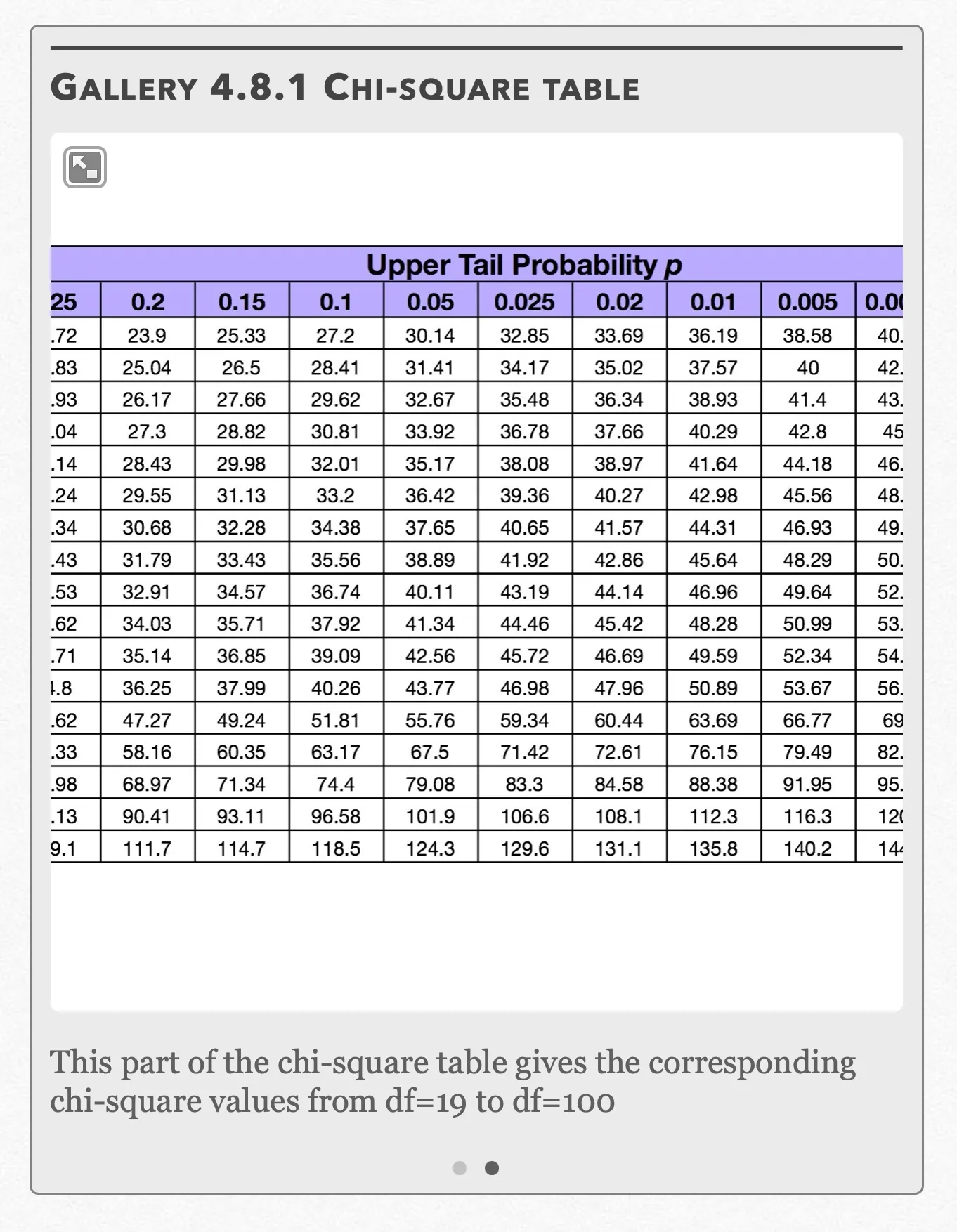
This part of the chi-square table gives the corresponding chi-square values from df=19 to df=100 Open full-size image S0483
Capture provenance
Filename capture times, with no recorded timezone. Frames above follow the original gallery positions.
- · S0482 · displayed frame 1
Screenshot 2026-10-05 at 4.07.25 PM.png - · S0483 · displayed frame 2
Screenshot 2026-10-05 at 4.07.30 PM.png
| Captured row | p=0.2 | p=0.15 | p=0.1 | p=0.05 | p=0.025 | p=0.02 | p=0.01 | p=0.005 |
|---|---|---|---|---|---|---|---|---|
| 1 | 1.64 | 2.07 | 2.71 | 3.84 | 5.02 | 5.41 | 6.63 | 7.88 |
| 2 | 3.22 | 3.79 | 4.61 | 5.99 | 7.38 | 7.82 | 9.21 | 10.6 |
| 3 | 4.64 | 5.32 | 6.25 | 7.81 | 9.35 | 9.84 | 11.34 | 12.84 |
| 4 | 5.99 | 6.74 | 7.78 | 9.49 | 11.14 | 11.67 | 13.28 | 14.86 |
| 5 | 7.29 | 8.12 | 9.24 | 11.07 | 12.83 | 13.39 | 15.09 | 16.75 |
| 6 | 8.56 | 9.45 | 10.64 | 12.59 | 14.45 | 15.03 | 16.81 | 18.55 |
| 7 | 9.8 | 10.75 | 12.02 | 14.07 | 16.01 | 16.62 | 18.48 | 20.28 |
| 8 | 11.03 | 12.03 | 13.36 | 15.51 | 17.53 | 18.17 | 20.09 | 21.95 |
| 9 | 12.24 | 13.29 | 14.68 | 16.92 | 19.02 | 19.68 | 21.67 | 23.59 |
| 10 | 13.44 | 14.53 | 15.99 | 18.31 | 20.48 | 21.16 | 23.21 | 25.19 |
| 11 | 14.63 | 15.77 | 17.28 | 19.68 | 21.92 | 22.62 | 24.72 | 26.76 |
| 12 | 15.81 | 16.99 | 18.55 | 21.03 | 23.34 | 24.05 | 26.22 | 28.3 |
| 13 | 16.98 | 18.2 | 19.81 | 22.36 | 24.74 | 25.47 | 27.69 | 29.82 |
| 14 | 18.15 | 19.41 | 21.06 | 23.68 | 26.12 | 26.87 | 29.14 | 31.32 |
| 15 | 19.31 | 20.6 | 22.31 | 25 | 27.49 | 28.26 | 30.58 | 32.8 |
| 16 | 20.47 | 21.79 | 23.54 | 26.3 | 28.85 | 29.63 | 32 | 34.27 |
| 17 | 21.61 | 22.98 | 24.77 | 27.59 | 30.19 | 31 | 33.41 | 35.72 |
| 18 | 22.76 | 24.16 | 25.99 | 28.87 | 31.53 | 32.35 | 34.81 | 37.16 |
| Captured row | p=0.2 | p=0.15 | p=0.1 | p=0.05 | p=0.025 | p=0.02 | p=0.01 | p=0.005 |
|---|---|---|---|---|---|---|---|---|
| 1 | 23.9 | 25.33 | 27.2 | 30.14 | 32.85 | 33.69 | 36.19 | 38.58 |
| 2 | 25.04 | 26.5 | 28.41 | 31.41 | 34.17 | 35.02 | 37.57 | 40 |
| 3 | 26.17 | 27.66 | 29.62 | 32.67 | 35.48 | 36.34 | 38.93 | 41.4 |
| 4 | 27.3 | 28.82 | 30.81 | 33.92 | 36.78 | 37.66 | 40.29 | 42.8 |
| 5 | 28.43 | 29.98 | 32.01 | 35.17 | 38.08 | 38.97 | 41.64 | 44.18 |
| 6 | 29.55 | 31.13 | 33.2 | 36.42 | 39.36 | 40.27 | 42.98 | 45.56 |
| 7 | 30.68 | 32.28 | 34.38 | 37.65 | 40.65 | 41.57 | 44.31 | 46.93 |
| 8 | 31.79 | 33.43 | 35.56 | 38.89 | 41.92 | 42.86 | 45.64 | 48.29 |
| 9 | 32.91 | 34.57 | 36.74 | 40.11 | 43.19 | 44.14 | 46.96 | 49.64 |
| 10 | 34.03 | 35.71 | 37.92 | 41.34 | 44.46 | 45.42 | 48.28 | 50.99 |
| 11 | 35.14 | 36.85 | 39.09 | 42.56 | 45.72 | 46.69 | 49.59 | 52.34 |
| 12 | 36.25 | 37.99 | 40.26 | 43.77 | 46.98 | 47.96 | 50.89 | 53.67 |
| 13 | 47.27 | 49.24 | 51.81 | 55.76 | 59.34 | 60.44 | 63.69 | 66.77 |
| 14 | 58.16 | 60.35 | 63.17 | 67.5 | 71.42 | 72.61 | 76.15 | 79.49 |
| 15 | 68.97 | 71.34 | 74.4 | 79.08 | 83.3 | 84.58 | 88.38 | 91.95 |
| 16 | 90.41 | 93.11 | 96.58 | 101.9 | 106.6 | 108.1 | 112.3 | 116.3 |
| 17 | 111.7 | 114.7 | 118.5 | 124.3 | 129.6 | 131.1 | 135.8 | 140.2 |
Example 4.8.1
In Example 4.1.1, we introduced Will it Mend?, a company that fixes all manner of items large and small. The following table provides data on the number of items repaired over the course of a randomly selected week within the last year under 7 different categories:
| Type of item | Observed Repairs (Count) |
|---|---|
| Appliances | 168 |
| Consumer Electronics | 189 |
| Toys | 81 |
| Apparel | 102 |
| Furniture | 47 |
| Auto | 61 |
| Other | 27 |
Will it Mend? claims that the percentage of items repaired follows the distribution as given in the table:
| Type of item | Expected Repairs (Percent) |
|---|---|
| Appliances | 0.20 |
| Consumer Electronics | 0.30 |
| Toys | 0.10 |
| Apparel | 0.15 |
| Furniture | 0.10 |
| Auto | 0.10 |
| Other | 0.05 |
Example 4.8.1 — source solution (a)
(a) First, we want to check our three conditions:
Random — The number of repairs came from a randomly selected week.
Large Sample Size — Due to the large number of repairs we’re dealing with in the problem, we should have no problem assuming that all of the expected counts are at least 5.
Independent — We are sampling without replacement, so Will it Mend will have to have repaired at least 10(675) = 6750 items. Although the exact number of repairs will likely differ from week-to-week, we had 52 week’s worth of repairs to pick from, so it is safe to assume that this condition will easily be met.
Since the data is organized in a one-way table, we use the Goodness of Fit Test. Our significance test is structured as follows:
H₀: Will it Mend’s stated distribution of repairs in the 7 possible categories is correct, or
Hₐ: Will it Mend’s stated distribution of repairs in the 7 possible categories is incorrect, or
one-way table is calculated as follows:
where
For instance, the expected count of appliances and other items respectively are calculated as:
And so on… Therefore, the chi-square statistic would look something like:
Gallery 4.8.2 Example 4.8.1 (one-way table chi-square test on TI-83/84)
Frame 1 of 8
Press the STAT button and under EDIT, select “Edit” and press ENTER Open full-size image S0486Frame 2 of 8
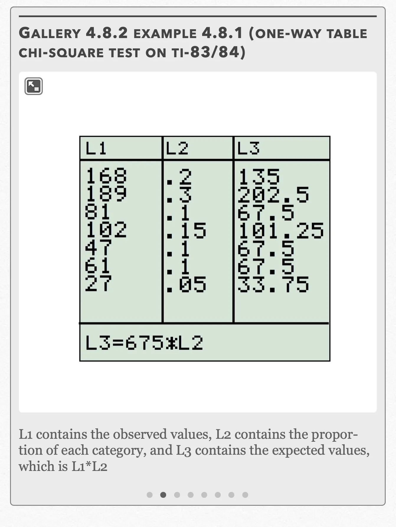
L1 contains the observed values, L2 contains the proportion of each category, and L3 contains the expected values, which is L1*L2 Open full-size image S0487Frame 3 of 8
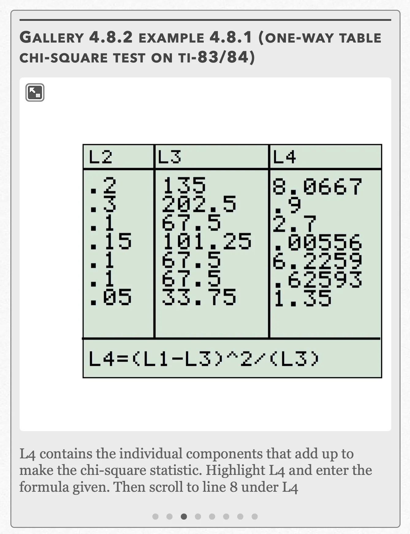
L4 contains the individual components that add up to make the chi-square statistic. Highlight L4 and enter the formula given. Then scroll to line 8 under L4 Open full-size image S0488Frame 4 of 8
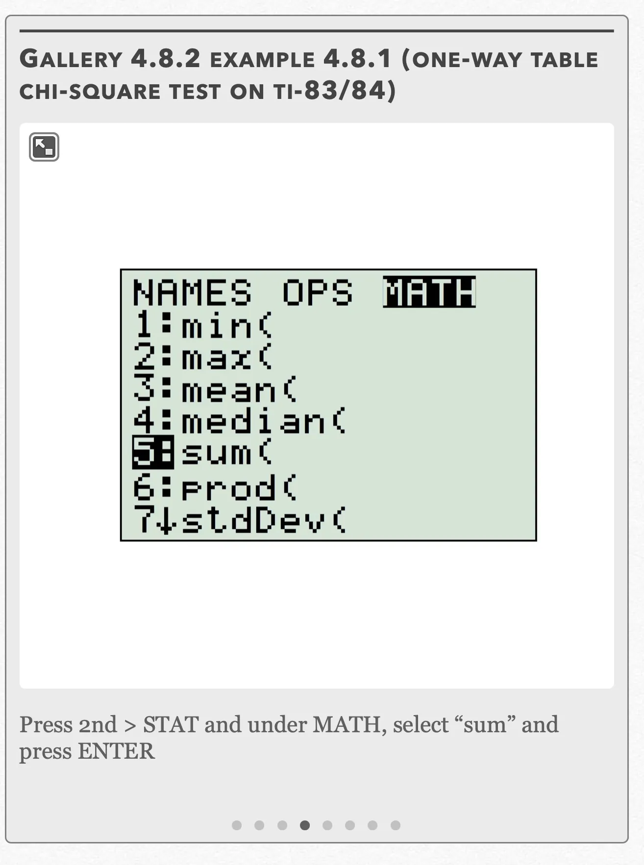
Press 2nd>STAT and under MATH, select “sum” and press ENTER Open full-size image S0489Frame 5 of 8
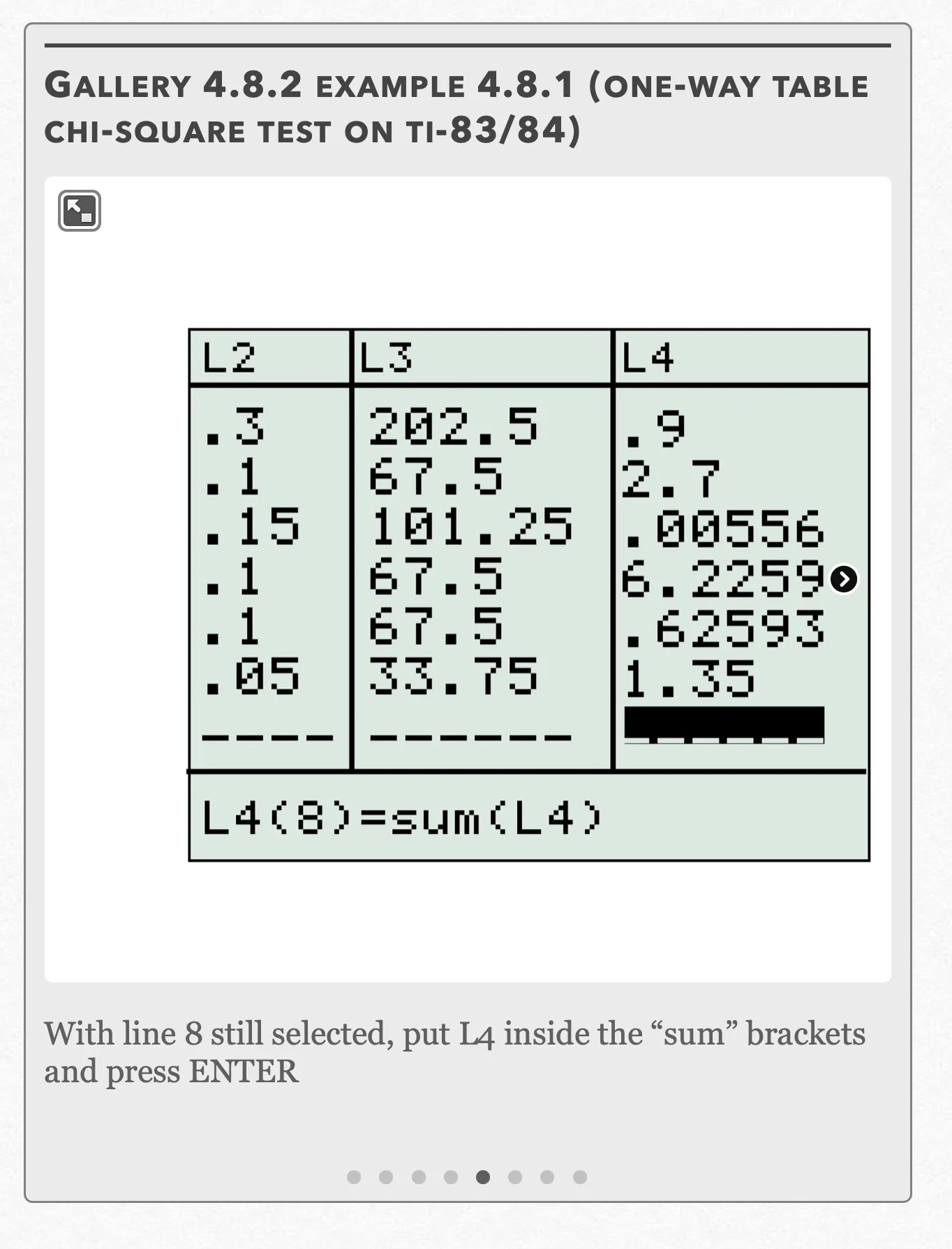
With line 8 still selected, put L4 inside the “sum” brackets and press ENTER Open full-size image S0490Frame 6 of 8
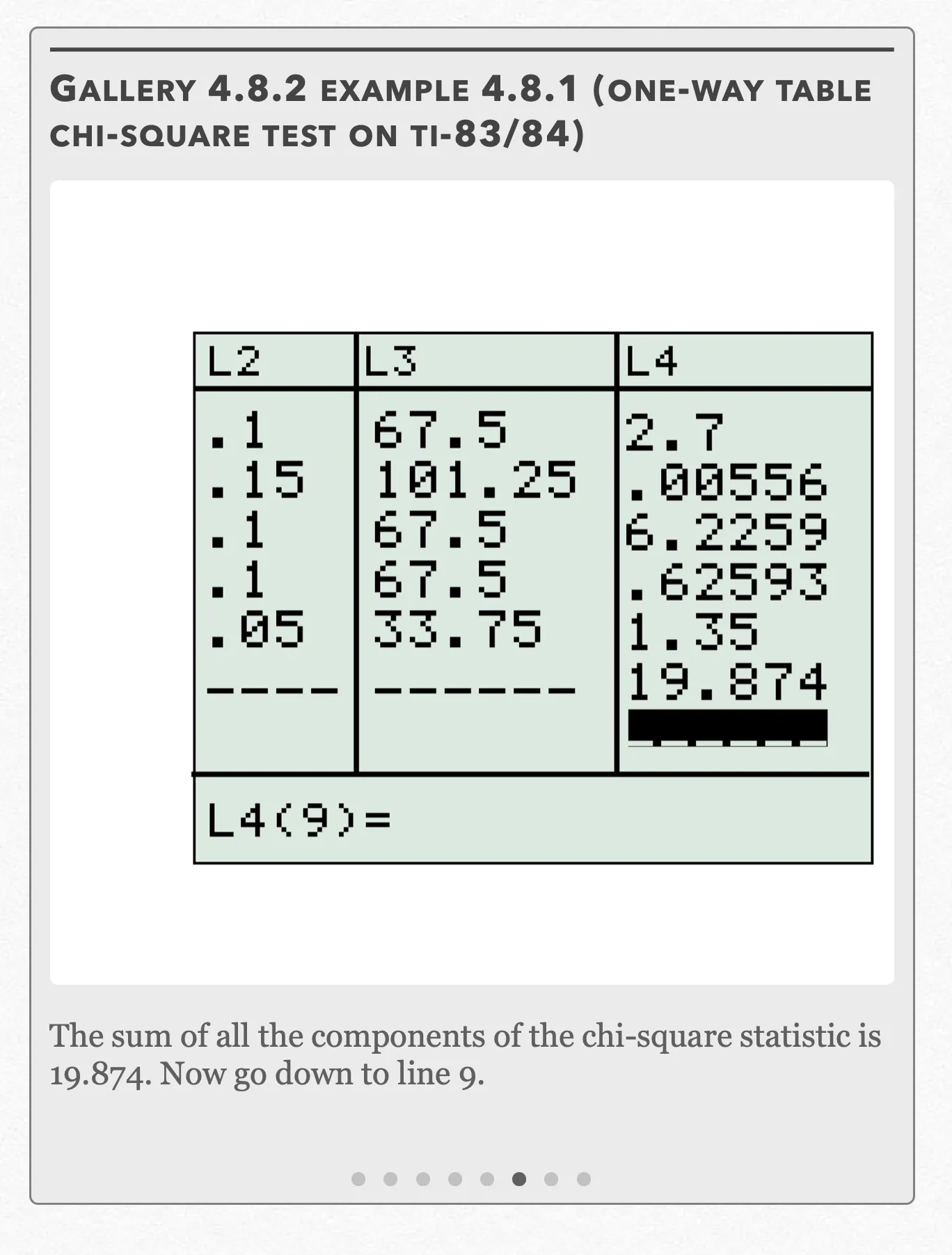
The sum of all the components of the chi-square statistic is 19.874. Now go down to line 9. Open full-size image S0491Frame 7 of 8
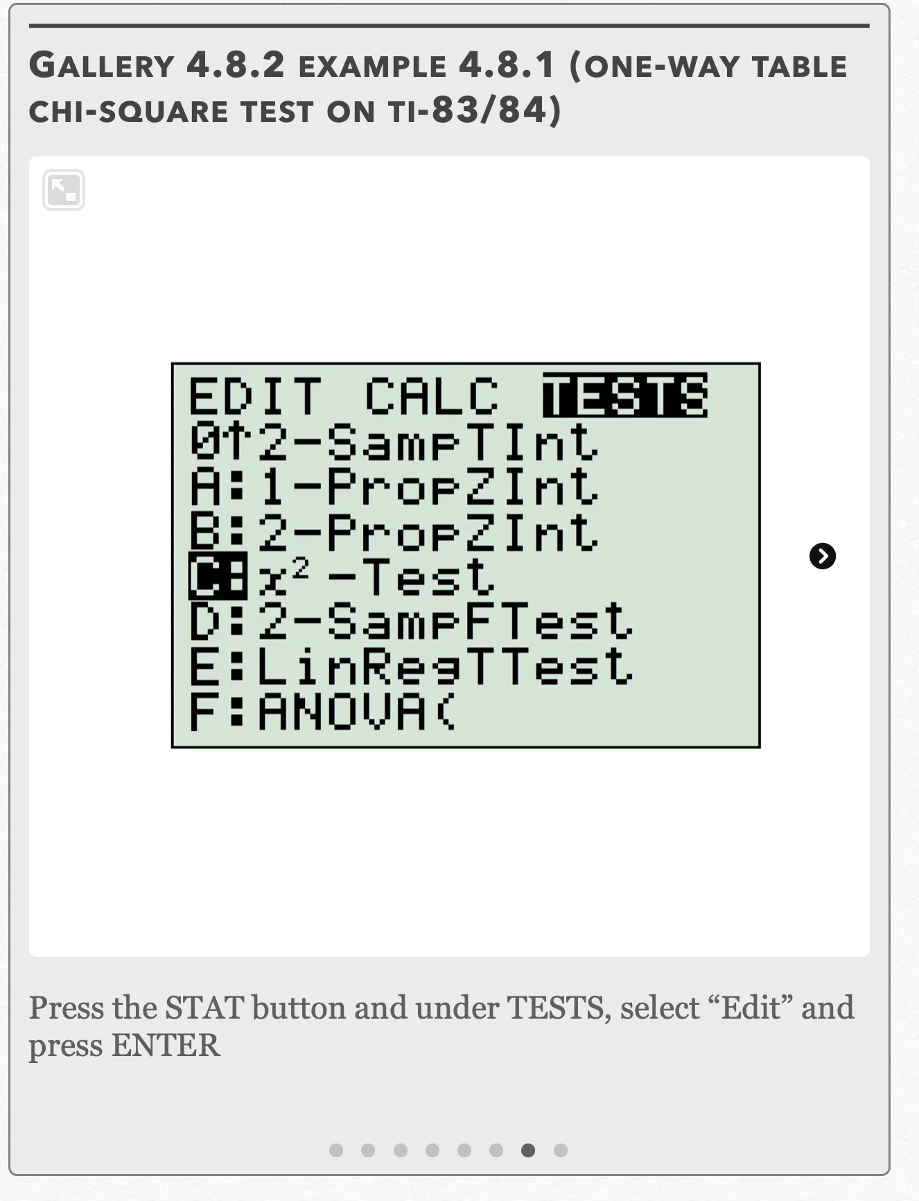
Press the STAT button and under TESTS, select “Edit” and press ENTER Open full-size image S0492Frame 8 of 8
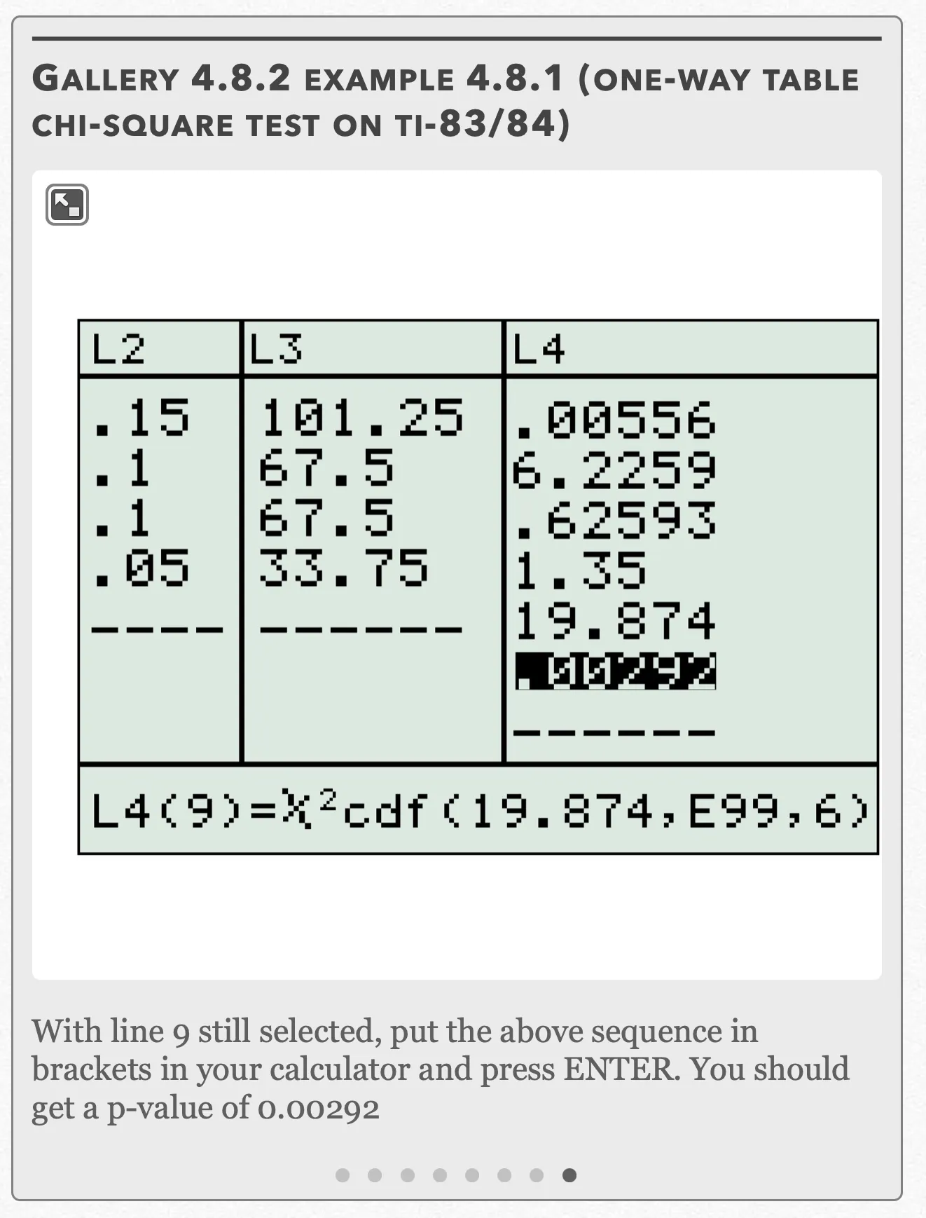
With line 9 still selected, put the above sequence in brackets in your calculator and press ENTER. You should get a p-value of 0.00292 Open full-size image S0493
Capture provenance
Filename capture times, with no recorded timezone. Frames above follow the original gallery positions.
- · S0486 · displayed frame 1
Screenshot 2026-10-05 at 4.07.34 PM.png - · S0487 · displayed frame 2
Screenshot 2026-10-05 at 4.07.38 PM.png - · S0488 · displayed frame 3
Screenshot 2026-10-05 at 4.07.44 PM.png - · S0489 · displayed frame 4
Screenshot 2026-10-05 at 4.07.47 PM.png - · S0490 · displayed frame 5
Screenshot 2026-10-05 at 4.07.51 PM.png - · S0491 · displayed frame 6
Screenshot 2026-10-05 at 4.07.55 PM.png - · S0492 · displayed frame 7
Screenshot 2026-10-05 at 4.07.59 PM.png - · S0493 · displayed frame 8
Screenshot 2026-10-05 at 4.08.02 PM.png
The visible calculator lists, in the original category order, are:
| Category | L1 observed | L2 proportion | L3 expected | L4 component |
|---|---|---|---|---|
| Appliances | 168 | 0.2 | 135 | 8.0667 |
| Consumer Electronics | 189 | 0.3 | 202.5 | 0.9 |
| Toys | 81 | 0.1 | 67.5 | 2.7 |
| Apparel | 102 | 0.15 | 101.25 | 0.00556 |
| Furniture | 47 | 0.1 | 67.5 | 6.2259 |
| Auto | 61 | 0.1 | 67.5 | 0.62593 |
| Other | 27 | 0.05 | 33.75 | 1.35 |
, which corresponds to a p-value of 0.0029
Refer to Gallery 4.8.2 for how to perform these steps on your calculator.
We want to compare the chi-square statistic to the critical chi-square value. To find the critical chi-square value, we need the upper tail probability and the degrees of freedom. The degrees of freedom for a chi-square statistic that relies on a one-way table is df = 7 − 1 = 6. The upper tail probability is 0.01. With these two pieces of information, we get a critical chi-square value of 16.81 according to the chi-square table.
We see that the chi-square statistic is greater than the critical chi-square value (19.874 > 16.81).
Alternatively, we see that the p-value is smaller than the significance level α (0.0029 < 0.01). Both results tell us that we can reject the null hypothesis and conclude that the proportion of repairs for each item category stated by Will it Mend? are probably not correct.
Example 4.8.1 — source solution (b)
b) Since our result in (a) was statistically significant, we can perform a follow-up analysis and examine the components that make up our chi-square statistic of 19.874. If we added our components manually, we see the components that make up most of the chi-square statistic are appliance repairs (8.067), toy repairs (2.7), and furniture repairs (6.226). These are the categories which deviated most from their respective observed counts. These values can also be found in L₄ on your calculator list screen (see Gallery 4.8.2).
Interactive 4.8.2 Example 4.8.1
Example 4.8.2
Recall in Chapter 1.1 that a MMORPG server surveyed players about their gender and character class. The results are shown in the following two-way table:
| Character class | Male | Female | Total |
|---|---|---|---|
| Knight | 752 | 403 | 1155 |
| Ninja | 611 | 445 | 1056 |
| Archer | 386 | 254 | 640 |
| Wizard | 460 | 655 | 1115 |
| Healer | 141 | 369 | 510 |
| Total | 2350 | 2126 | 4476 |
Back when we solved this example problem, we noted that there was a possible association between the player’s gender and class type. However, now we have the means to quantitatively see if our intuition was true.
Example 4.8.2 — source solution (a)
(a) First, we want to check our three conditions:
Random — The players were randomly chosen to take part in the survey.
Large Sample Size — Due to the large number of players we’re dealing with in the problem, we should have no problem assuming that all of the expected counts are at least 5.
Independent — We are sampling without replacement, so the server has to have at least 10(4476) = 44760 people on it. Although we know the exact number of total players on the server, we can assume it’s at least 44760 if the survey was given to only a “very small number of select players” as was mentioned initially in Chapter 1.1.
Since the data comes from one random sample, the appropriate chi-square test to use for this example is the Chi-Square Test of Association. Our significance test is structured as follows:
H₀: There is no association between gender and character class in the population of players on the server.
Hₐ: There is an association between gender and character class in the population of players on the server.
The chi-square statistic that relies on the two-way table is calculated as follows:
where
The expected count of male knights is calculated as:
The expected count of female healers is calculated as:
Gallery 4.8.3 Example 4.8.2 (two-way table chi-square test on TI-83/84)
Frame 1 of 4
Press 2nd>x⁻¹, go to EDIT, choose “[A]” and press ENTER Open full-size image S0497Frame 2 of 4
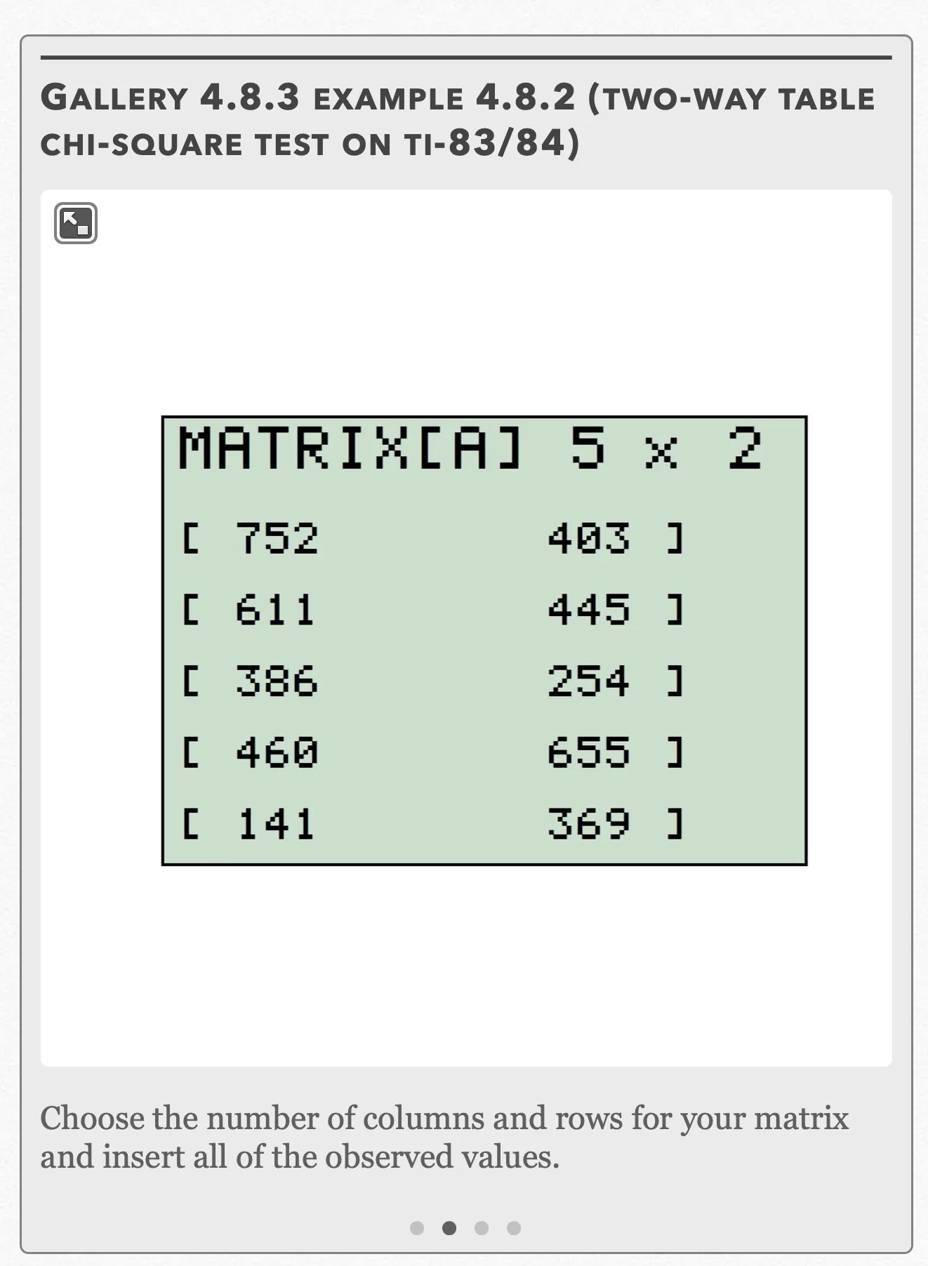
Choose the number of columns and rows for your matrix and insert all of the observed values. Open full-size image S0498Frame 3 of 4
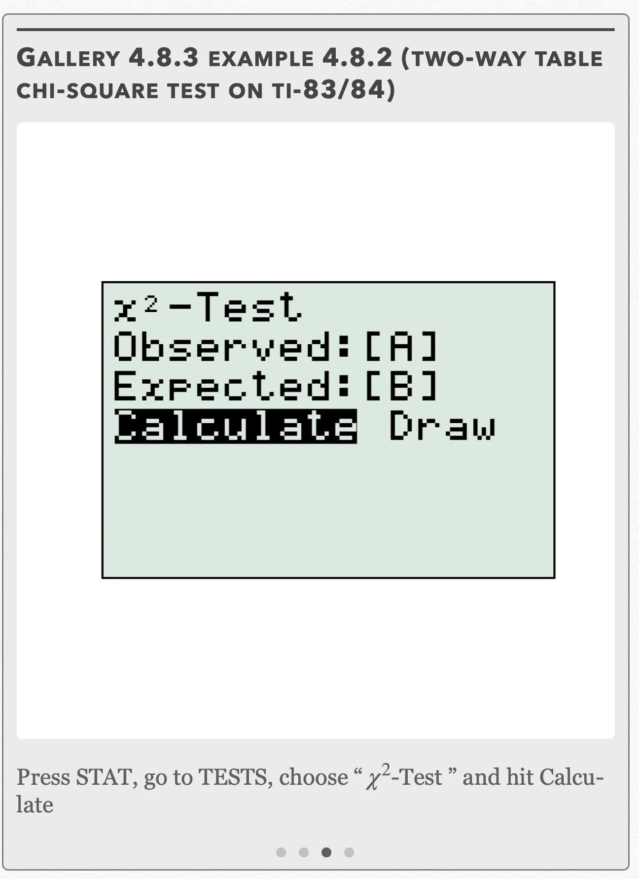
Press STAT, go to TESTS, choose “χ²-Test” and hit “Calculate” Open full-size image S0499Frame 4 of 4
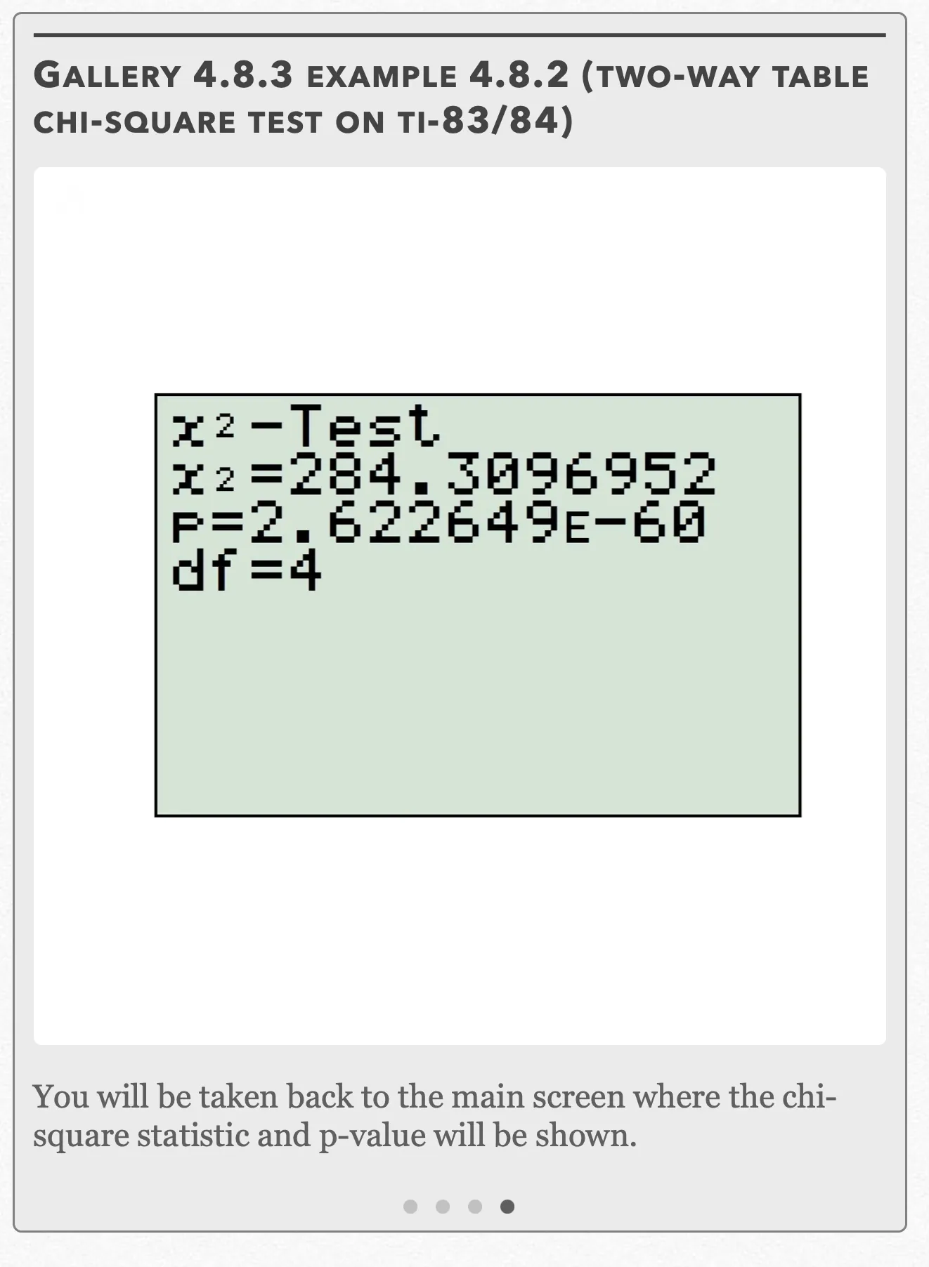
You will be taken back to the main screen where the chi-square statistic and p-value will be shown. Open full-size image S0500
Capture provenance
Filename capture times, with no recorded timezone. Frames above follow the original gallery positions.
- · S0497 · displayed frame 1
Screenshot 2026-10-05 at 4.08.08 PM.png - · S0498 · displayed frame 2
Screenshot 2026-10-05 at 4.08.12 PM.png - · S0499 · displayed frame 3
Screenshot 2026-10-05 at 4.09.23 PM.png - · S0500 · displayed frame 4
Screenshot 2026-10-05 at 4.09.27 PM.png
And so on… Therefore, the chi-square statistic would look something like:
, which corresponds to a p-value of
Refer to Gallery 4.8.3 for how to perform these steps on your calculator.
We want to compare the chi-square statistic to the critical chi-square value. To find the critical chi-square value, we need the upper tail probability and the degrees of freedom.
The degrees of freedom for a chi-square statistic that relies on a two-way table is
The upper tail probability is 0.10. With these two pieces of information, we get a critical chi-square value of 7.78 according to the chi-square table.
We see that the chi-square statistic is much greater than the critical chi-square value (284.31 > 7.78). Alternatively, we see that the p-value that corresponds to the chi-square statistic is much smaller than α (). Both results tell us that we can reject the null hypothesis and conclude that there is indeed an association between the player’s gender and their character class.
Example 4.8.2 — source solution (b)
Gallery 4.8.4 Example 4.8.2 (two-way table chi-square components on TI-83/84)
Frame 1 of 8
Press 2nd>x⁻¹, go to MATH, choose “Matr>List” and press ENTER Open full-size image S0502Frame 2 of 8
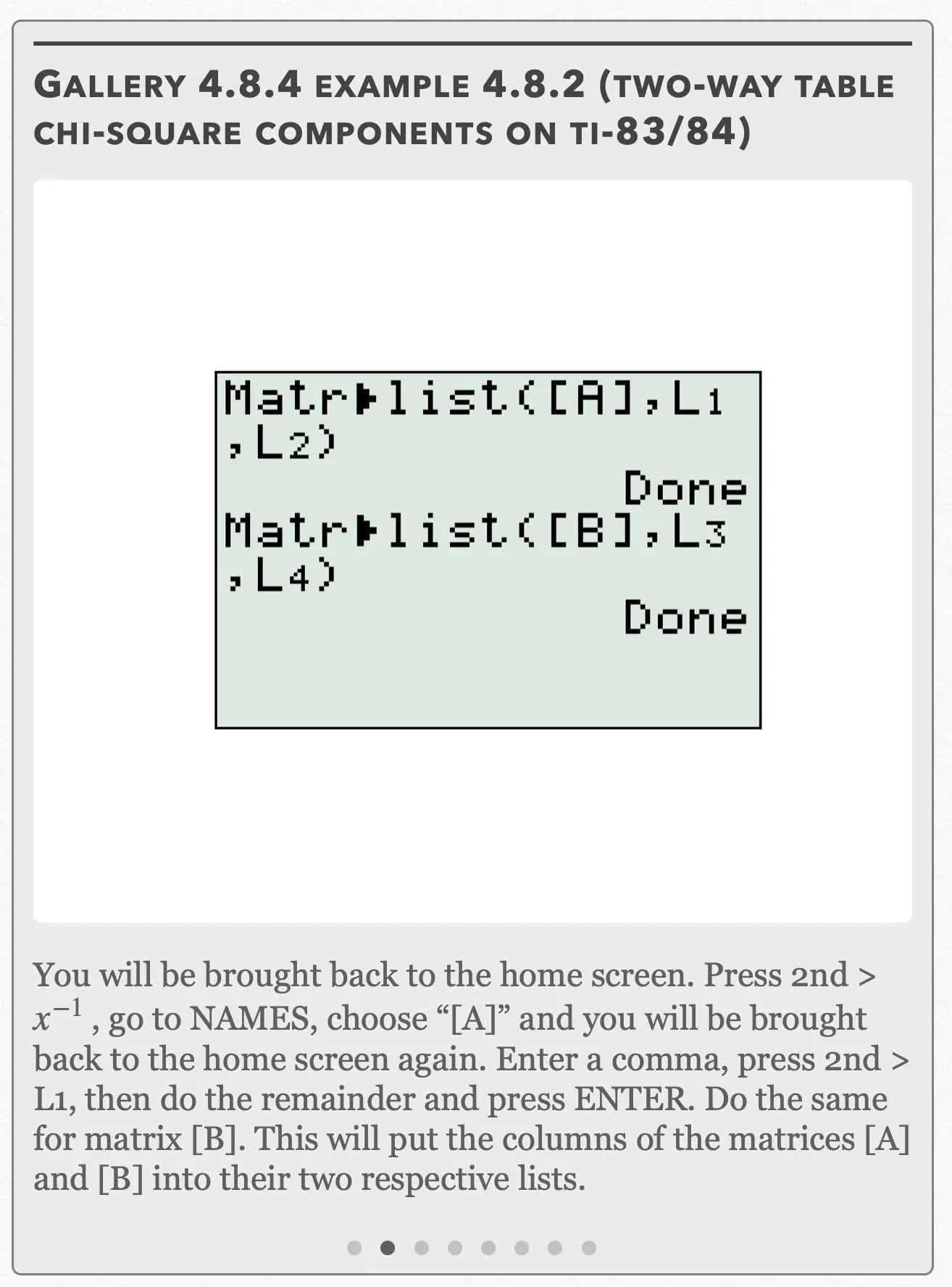
You will be brought back to the home screen. Press 2nd>x⁻¹, go to NAMES, choose “[A]” and you will be brought back to the home screen again. Enter a comma, press 2nd>L1, then do the remainder and press ENTER. Do the same for matrix [B]. This will put the columns of the matrices [A] and [B] into their two respective lists. Open full-size image S0503Frame 3 of 8
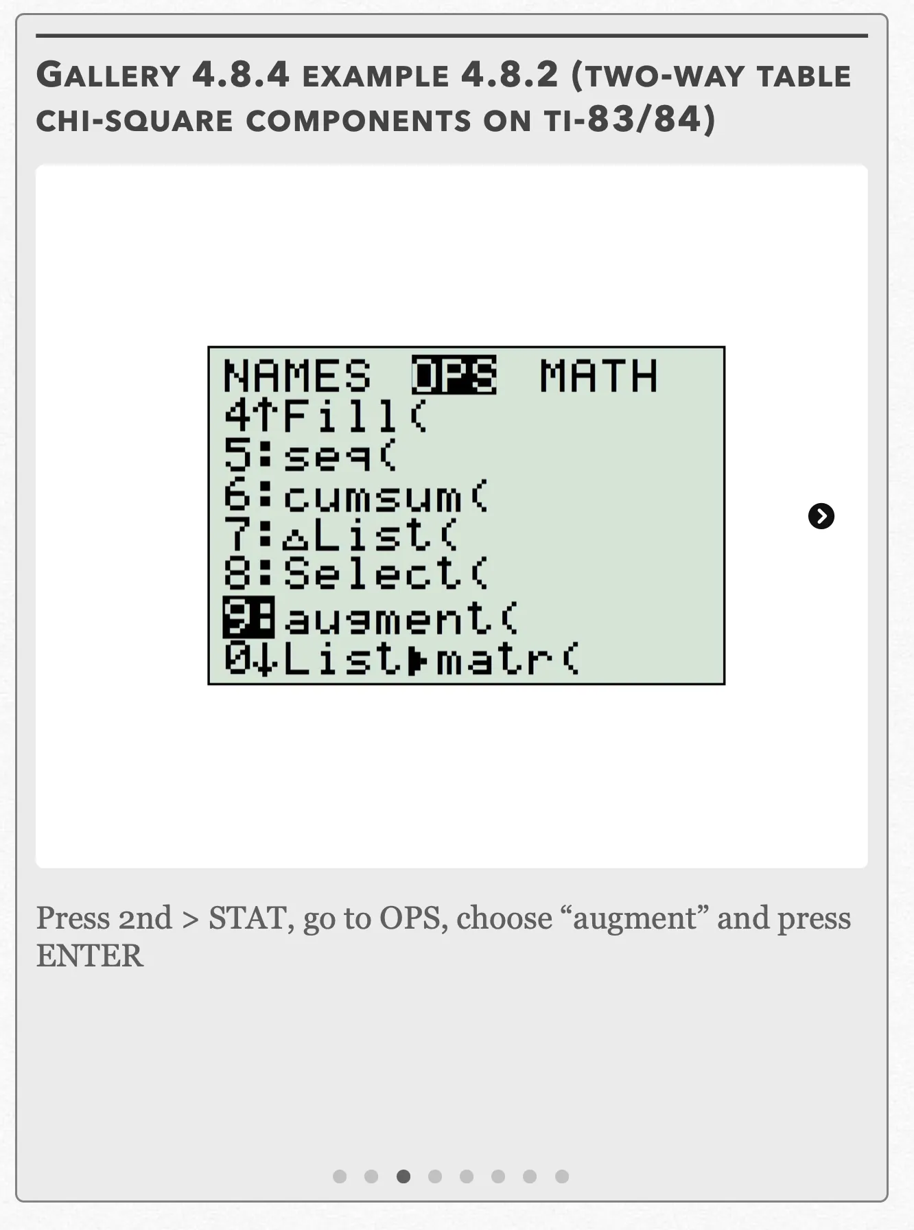
Press 2nd>STAT, go to OPS, choose “augment” and press ENTER Open full-size image S0504Frame 4 of 8
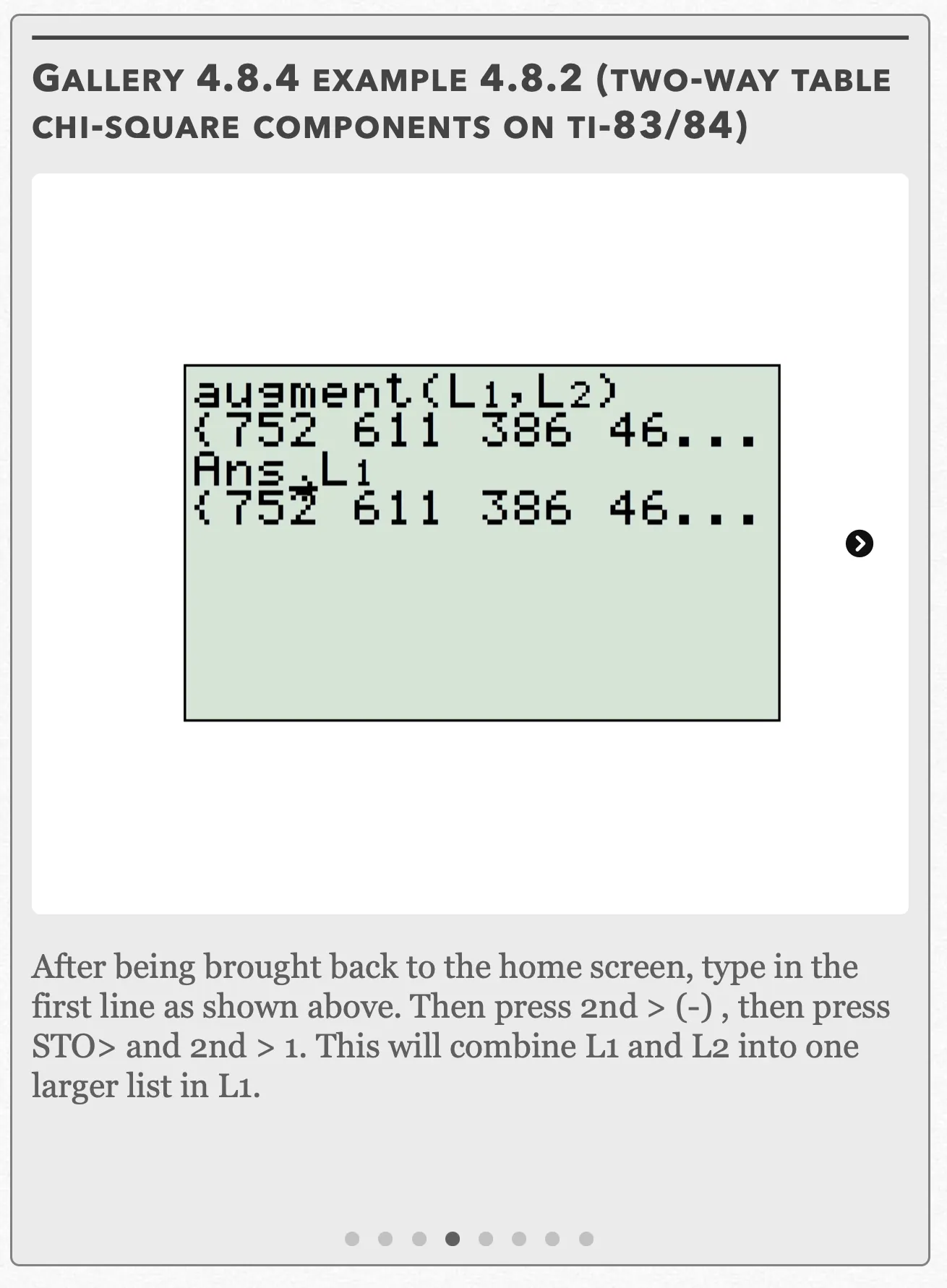
After being brought back to the home screen, type in the first line as shown above. Then press 2nd>(-), then press STO> and 2nd>1. This will combine L1 and L2 into one larger list in L1. Open full-size image S0505Frame 5 of 8
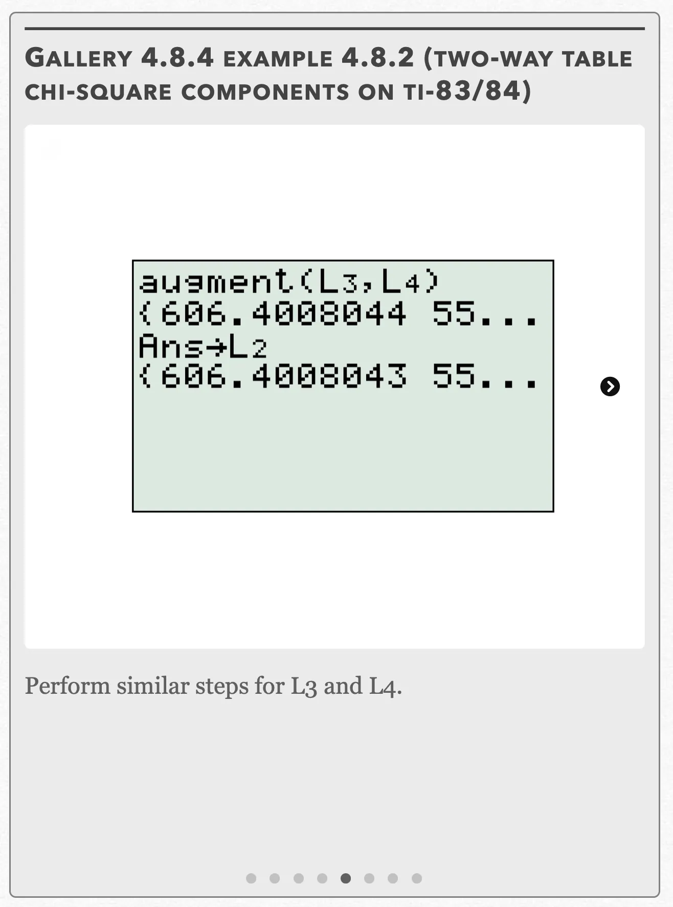
Perform similar steps for L3 and L4. Open full-size image S0506Frame 6 of 8
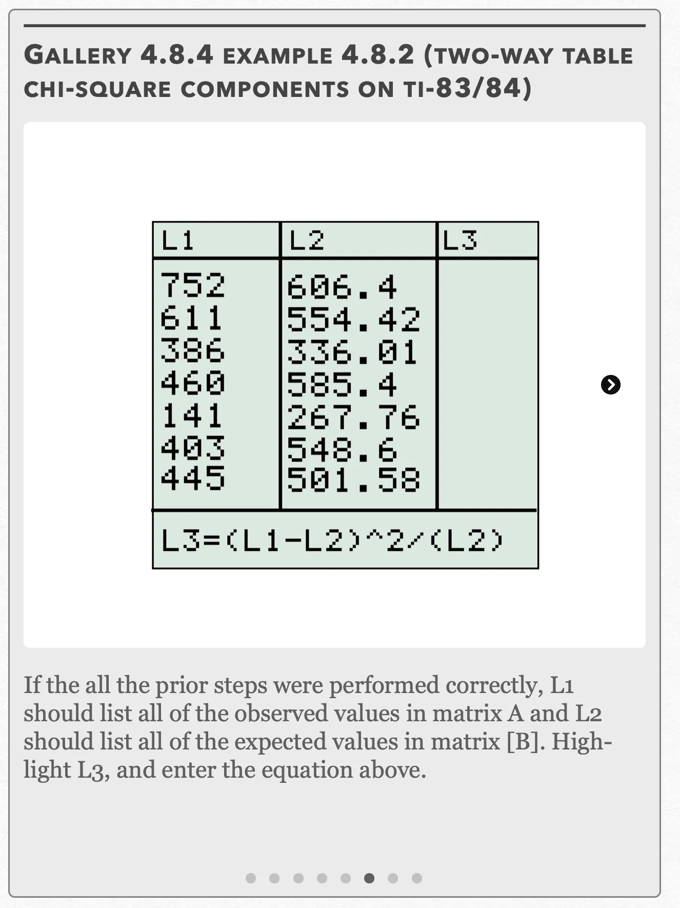
If the all the prior steps were performed correctly, L1 should list all of the observed values in matrix A and L2 should list all of the expected values in matrix [B]. Highlight L3, and enter the equation above. Open full-size image S0507Frame 7 of 8
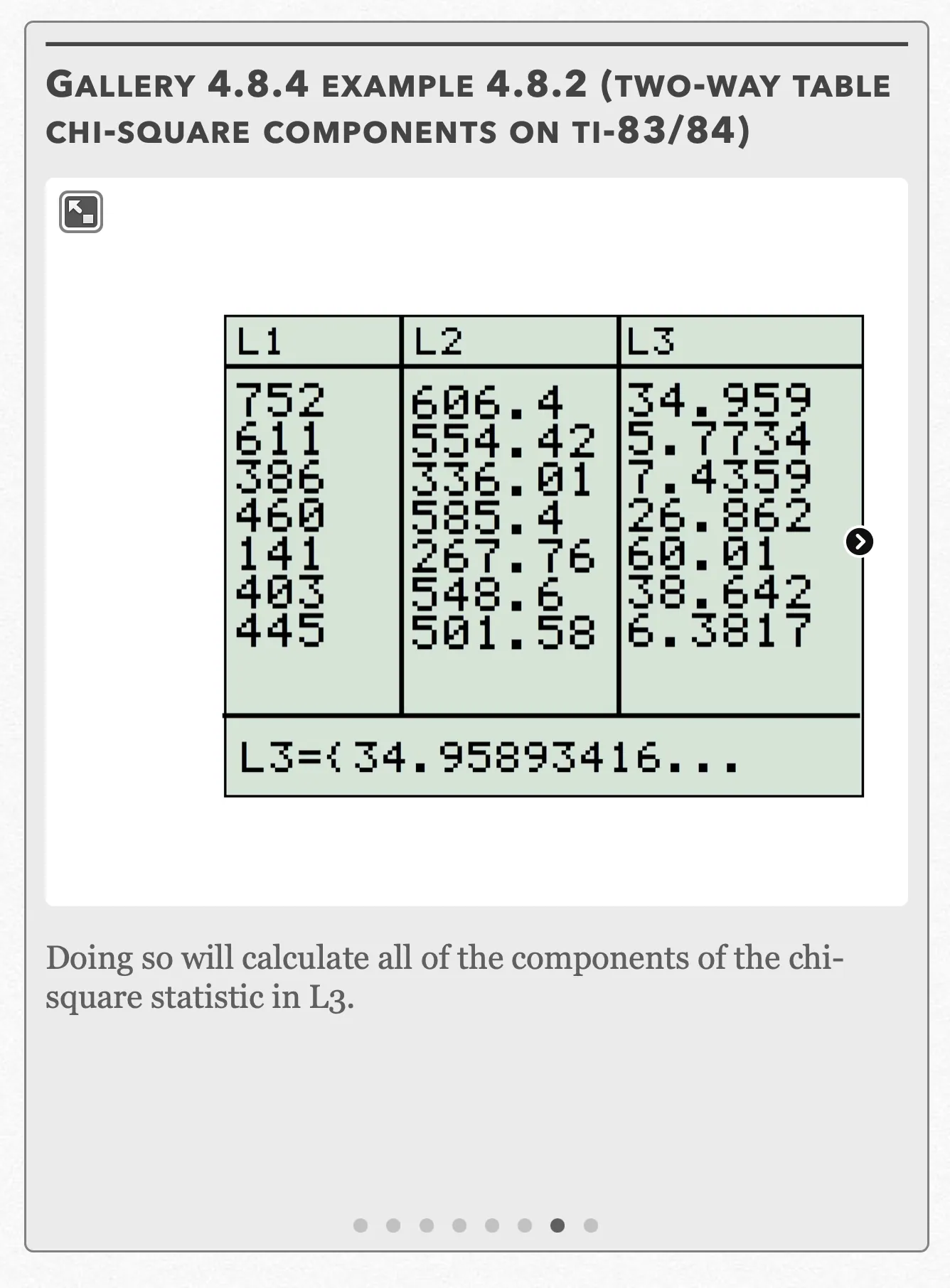
Doing so will calculate all of the components of the chi-square statistic in L3. Open full-size image S0508Frame 8 of 8
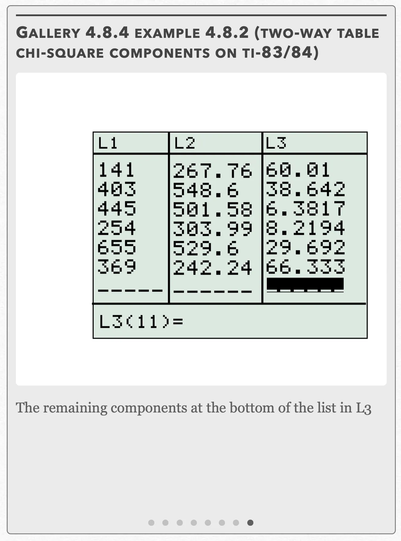
The remaining components at the bottom of the list in L3 Open full-size image S0509
Capture provenance
Filename capture times, with no recorded timezone. Frames above follow the original gallery positions.
- · S0502 · displayed frame 1
Screenshot 2026-10-05 at 4.09.33 PM.png - · S0503 · displayed frame 2
Screenshot 2026-10-05 at 4.09.37 PM.png - · S0504 · displayed frame 3
Screenshot 2026-10-05 at 4.09.41 PM.png - · S0505 · displayed frame 4
Screenshot 2026-10-05 at 4.09.45 PM.png - · S0506 · displayed frame 5
Screenshot 2026-10-05 at 4.09.49 PM.png - · S0507 · displayed frame 6
Screenshot 2026-10-05 at 4.09.53 PM.png - · S0508 · displayed frame 7
Screenshot 2026-10-05 at 4.09.56 PM.png - · S0509 · displayed frame 8
Screenshot 2026-10-05 at 4.10.01 PM.png
(b) Since our result in (a) was statistically significant, we can perform a follow-up analysis and examine the components that make up our chi-square statistic of value 284.31. If we added our components manually, we see the components that make up most of the chi-square statistic are the male knights (34.959), female ninjas (26.862), male archers (60.01), female archers (38.642), male healers (29.692), and female healers (66.333). These are the cells which deviated most from their respective observed counts. These values can also be found in L3 on your calculator list screen (see Gallery 4.8.4.)
| Cell in original matrix order | L1 observed | L2 expected | L3 component |
|---|---|---|---|
| Male Knight | 752 | 606.4 | 34.959 |
| Male Ninja | 611 | 554.42 | 5.7734 |
| Male Archer | 386 | 336.01 | 7.4359 |
| Male Wizard | 460 | 585.4 | 26.862 |
| Male Healer | 141 | 267.76 | 60.01 |
| Female Knight | 403 | 548.6 | 38.642 |
| Female Ninja | 445 | 501.58 | 6.3817 |
| Female Archer | 254 | 303.99 | 8.2194 |
| Female Wizard | 655 | 529.6 | 29.692 |
| Female Healer | 369 | 242.24 | 66.333 |
Pop Quiz 4.8.1
Glossary and deeper reading · 23 refreshers
These editorial refreshers supplement the reading. Definitions and examples are added guidance; original source wording and recorded answers remain in their original context.
-
Statistical inference
Statistical inference uses data and a study design to draw conclusions beyond the observed values. Random sampling supports population generalization, while well-conducted random assignment supports treatment-effect conclusions. For example, a random sample can estimate a school-wide preference without surveying every student.
Read more: Statistical inference in the captured Statistics reading →
-
Quantitative variable
A quantitative variable records a numerical count or measurement for each individual. Differences between its values have a meaningful numerical interpretation. For example, the number of books borrowed and the mass of a backpack are quantitative variables.
Read more: Quantitative variable in the captured Statistics reading →
-
Chi-square testing
Chi-square categorical tests compare observed counts with expected counts under a null model. The appropriate test depends on the study design, categorical variables, and hypothesis, with independence and expected-count conditions checked. For example, one sample with two categorical variables can be analyzed for association using a two-way table.
Read more: Chi-square testing in the current two-way chi-square lesson →
-
One-way table
A one-way table lists counts or proportions for the categories of one variable. The categories should cover the intended outcomes without overlap. For example, a table listing counts for walking, cycling, and riding describes one transportation variable.
-
Degrees of freedom
Degrees of freedom describe the independent information remaining after constraints or estimated quantities are accounted for. The value depends on the procedure, rather than always being the sample size minus 1. For example, a one-sample t procedure uses n − 1 degrees of freedom, while simple regression inference uses n − 2.
Read more: Degrees of freedom in the captured Statistics reading →
-
Alternative hypothesis
An alternative hypothesis specifies the population difference or direction for which a test seeks evidence. It should be chosen from the research question before inspecting results. For example, an alternative can state that the population mean travel time is greater than 15 minutes.
Read more: Alternative hypothesis in the captured Statistics reading →
-
Categorical variable
A categorical variable records a group or label for each individual. Numeric labels still count as categories when arithmetic on them has no meaningful interpretation. For example, favorite school subject is categorical, even if each subject receives a numbered code.
Read more: Categorical variable in the captured Statistics reading →
-
Two-way table
A two-way table organizes counts for combinations of two categorical variables. The cells show combinations, while row and column totals summarize each variable separately. For example, a table can classify students by grade level and whether they walk to school.
Read more: Two-way table in the captured Statistics reading →
-
Chi-square test for homogeneity
A chi-square test for homogeneity compares a categorical variable’s distribution across independently sampled populations or randomized treatment groups. The null model states that the category proportions are the same across groups. For example, independently sampled students at several schools can be compared for their transportation-mode distributions.
Read more: Chi-square test for homogeneity in the current two-way chi-square lesson →
-
Expected count
An expected count is the count predicted for a category or cell under the null model. Goodness-of-fit expectations use the total count times the null proportion, while independence-table expectations use row total times column total divided by the grand total. For example, a null proportion of 0.2 in 50 trials gives an expected count of 10.
Read more: Expected count in the current two-way chi-square lesson →
-
Distribution of data
A distribution describes the values a variable takes and how often those values occur. For quantitative data, useful features include shape, center, spread, and unusual observations. For example, a distribution of commuting times shows which times are common and how widely they vary.
Read more: Distribution of data in the captured Statistics reading →
-
Treatment
A treatment is a specific condition imposed on an experimental unit. In a multifactor experiment, a treatment is a combination of factor levels. For example, low fertilizer with eight hours of light is one treatment combination.
-
Chi-square test of association
A chi-square test of association examines the relationship between two categorical variables measured on one sample. The null model states that the variables are independent in the population. For example, one random sample of students can be classified by grade level and transportation mode to investigate association.
Read more: Chi-square test of association in the current two-way chi-square lesson →
-
Random sampling
Random sampling uses a specified chance process to select individuals from a population. It supports population inference when the sampling frame and data collection are appropriate, but does not guarantee perfect balance or eliminate every source of bias. For example, a random-number generator can select student identifiers from an enrollment list.
Read more: Random sampling in the captured Statistics reading →
-
Experiment
An experiment deliberately imposes treatments and measures responses. Random assignment, comparison, and replication help distinguish treatment effects from other variation. For example, assigning plants to fertilizer treatments is an experiment.
-
Sample
A sample is the subset of a population actually studied. How it is selected matters for the conclusions that can be drawn about the population. For example, 60 selected students may be a sample from a school’s full enrollment.
-
Statistical independence
Statistical independence means that learning one outcome does not change the probability distribution of another. For two events, it implies that the probability of both occurring equals the product of their probabilities. For example, independent draws with replacement keep the second draw’s color probabilities unchanged by the first.
Read more: Statistical independence in the captured Statistics reading →
-
Observation
An observation is a recorded value or set of values for an individual or occasion. The individual may be a person, object, or event rather than a human subject. For example, one plant’s measured height is an observation in a plant-growth study.
-
Chi-square statistic
For categorical-count tests, the chi-square statistic adds each cell’s squared observed-minus-expected difference divided by its expected count. Large contributions identify cells with substantial discrepancies relative to their expected counts. For example, a cell observed 15 times when 10 are expected contributes 2.5 to the statistic.
Read more: Chi-square statistic in the current two-way chi-square lesson →
-
Statistical significance
A result is statistically significant at a stated level when it meets the test’s rejection rule. Statistical significance alone does not establish a large effect, practical importance, or causation. For example, a very large sample can detect a small population difference that has little practical importance.
Read more: Statistical significance in the captured Statistics reading →
-
Chi-square component
A chi-square component is one cell’s contribution to a categorical test’s total chi-square statistic. Examining components can show which cells disagree most with the null expectations, without automatically establishing a new significant comparison. For example, a particularly large component highlights a category worth further contextual investigation.
Read more: Chi-square component in the current two-way chi-square lesson →
-
Critical value
A critical value is a cutoff from a reference distribution chosen for a confidence level or testing rule. The relevant distribution, degrees of freedom, and one-sided or two-sided procedure determine the cutoff. For example, a symmetric 95% Normal interval uses a cutoff near 1.96 standard-error units.
Read more: Critical value in the captured Statistics reading →
-
Probability
Probability quantifies how likely an event is under a specified chance model. It lies between 0 and 1, with larger values representing greater likelihood. For example, drawing a red card from a well-shuffled standard deck has probability one half.