Describe a Quantitative Distribution in Context

A quantitative plot is more than a collection of dots or bars. A description should help someone imagine the pattern and understand what it means for the measured people or things. Start with shape, center, and variability, then call attention to features that would be missed by a single average.

Describe Shape, Center, and Spread

Shape concerns the overall pattern. A right-skewed, or positively skewed, distribution has a longer tail toward larger values than toward smaller values. A left-skewed, or negatively skewed, distribution has a longer tail toward smaller values. An approximately symmetric distribution has left and right halves that are roughly mirror images. Judge the tails, not merely which side contains the tallest bar.

A unimodal distribution has one main peak; bimodal has two prominent peaks. An approximately uniform distribution has frequencies or relative frequencies about the same across its values or intervals, without prominent peaks. A small bump is not automatically a meaningful second mode; the representation and overall pattern matter.

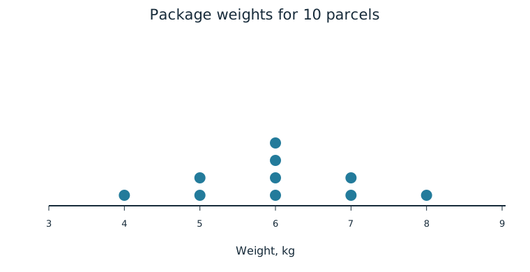
Describe a typical location as the center and the amount of variation as spread. For the parcel plot, a typical weight is around 6 kg and observed weights run from 4 to 8 kg. Both statements name the variable and units. A description saying “center 6 and spread 4” leaves a reader to guess what was measured and whether 4 means range, standard deviation, or something else.

Unusual features include outliers, unusually small or large values relative to the rest; gaps, intervals between values containing no observations; and clusters, concentrations of observations usually separated by gaps. A gap is not a missing record invented to make the graph smooth. It is a feature of the observed distribution. An isolated value can suggest a possible outlier before a formal numerical rule is applied.

Worked Example: Service Times

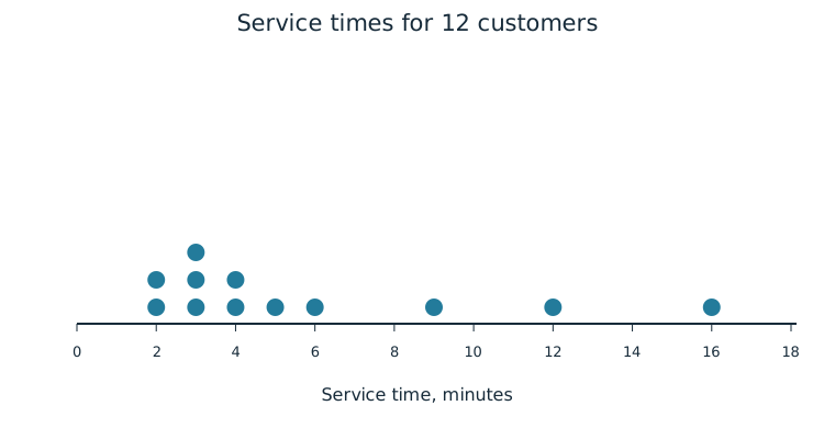
These sampled service times are right-skewed and have a main concentration around 2–4 minutes. Most waits are under 7 minutes, but observations extend to 16 minutes; the spread is substantial relative to a typical time. The long right tail makes “everyone was served quickly” a poor description. If a point seems isolated, say why it stands apart and whether it is only a possible outlier or has also met a stated numerical rule.

Justify With Visible Features

A plot can support a contextual claim when the claim follows from its features. To assess “parcel weights are roughly balanced around 6 kg,” point to the matched counts at equal distances from 6. To assess “no customer waited more than 10 minutes” in the service plot, the 12- and 16-minute observations refute it. Use numerical positions, counts, tails, or clusters as evidence.

Do not confuse a description of the observed sample with a claim about every future observation. A symmetric sample does not ensure the next parcel weighs 6 kg. A plotted association or shape also does not reveal the cause of that pattern. The graph makes the data visible; the argument must stay within what the data and study support.

Independent Practice

Use the information in each question to make your own calculation, representation, or argument. Explain what your result means in its setting.

Original generated practice for the Fall 2026 course.

Describe community-room setup times

Nine measured setup times for a community room, in minutes, are 9,10,10,11,11,11,12,12,13. The dotplot represents every observation.

Part a

Describe shape, approximate center, and observed spread in context. Use specific matching values and their frequencies on opposite sides of the center to justify your shape description, and identify any main peak.

Your reasoning

Worked answer and rubric

Name the longer tail

Part a

Describe each skew direction and explain using the tail toward larger or smaller values.

Your reasoning

Worked answer and rubric

Peaks and flatness

Equal-width histogram bins in increasing measurement order; bar heights given.

Bin midpoint	Plot U frequency	Plot B frequency	Plot F frequency
1	1	4	3
2	3	1	3
3	6	1	3
4	3	1	3
5	1	4	3

Part a

Describe which histogram is unimodal, bimodal, or uniform. Explain the frequency pattern in each.

Your reasoning

Worked answer and rubric

Refute a universal claim

Part a

Justify or reject “every sampled customer was served in at most 10 minutes.” Identify graphical evidence and a limit on future claims.

Your reasoning

Worked answer and rubric

Tell the story of tour waits

Part a

Describe the distribution’s shape, approximate center, and observed variability in context. Include its prominent peaks.

Your reasoning

Part b

Identify the clusters, at least one gap, and a possible outlier. Explain what each term means using this plot.

Your reasoning

Part c

Justify or reject “all visitors waited less than 20 minutes” and “most sampled waits were below 10 minutes.” Give counts from the graph.

Your reasoning

Part d

Explain why describing this as an approximately uniform distribution would be misleading.

Your reasoning

Worked answer and rubric