2.1 Seeing Relationships Between Categorical Variables

Two Labels for Each Person

At a community workshop, each participant has two categorical labels: membership status and workshop time. A two-way table, also called a contingency table, preserves their relationship. Each interior cell counts participants with both labels. Entries can be frequencies (counts) or relative frequencies (proportions); always check which kind is shown.

	Day	Evening	Weekend	Total
Member	20	10	10	40
Nonmember	10	30	20	60
Total	30	40	30	100

The table is complete for these 100 participants. Its 20 in the first cell describes members attending by day, not all members and not all day participants. Dividing every cell by 100 would make a joint-relative-frequency table without changing the underlying data.

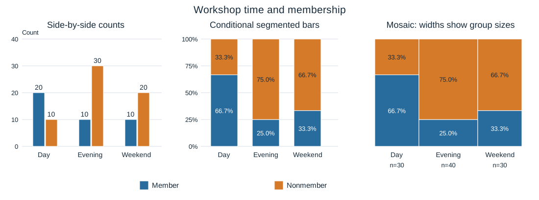
Three graphs can display the same relationship in different ways. In a side-by-side bar chart, member and nonmember counts sit next to one another at each time. A segmented bar chart splits a same-height bar into conditional proportions: each time’s participants total 100%. A mosaic plot also splits each time into proportions, but gives larger groups more width. In this mosaic, area is proportional to the joint relative frequency.

Worked Comparison: Counts or Composition?

The side-by-side chart answers “How many?” Evening has the most participants, 40, and 30 of them are nonmembers. The segmented chart answers “What proportion within each time?” The member proportions are $20/30\approx66.7\%$ for Day, $10/40=25\%$ for Evening and $10/30\approx33.3\%$ for Weekend. The mosaic preserves these heights and shows Evening’s larger group with a wider column.

These differences support an association between membership and workshop time in this participant population. The membership distributions are not the same across the time categories. A member is a much larger share of Day attendees than of Evening attendees. The table supplies the denominators; the conditional bars make the distribution differences immediately visible.

Suppose someone claims, “The larger Evening group means Evening has the largest proportion of members.” The claim confuses a total with a composition. The table has only 10 Evening members among 40 Evening participants, versus 20 among 30 Day participants. The displayed conditional proportions reject the claim. A useful justification names the groups, gives the relevant numbers and connects them to the claim; it does not merely say a graph “looks different.”

The plots have distinct strengths. Counts retain group size; segmented bars make proportions easier to compare; mosaic widths retain group sizes while heights show composition. No representation adds new observations. Also, this association alone does not establish that changing a participant’s membership would cause a different workshop-time choice. Keep the conclusion tied to the variables and participants actually represented.

Try It Yourself

The following original practice applies the ideas above to a fresh setting. Show the reasoning requested in each part. Answers and task-specific rubrics are on the separate solutions page.

Original generated practice for the Fall 2026 course.

Compare Four Views of the Same Survey

Complete survey population of 120 students

Club attendance	Walk	Bus	Car	Total
Attends	30	20	10	60
Does not attend	10	30	20	60
Total	40	50	30	120

Each student has exactly one commute mode and one club-attendance label. This table and its three graphs describe all 120 surveyed students.

Part a

Compare the table with the side-by-side graph. Identify what the entries and bar heights represent; give one matching numerical example. Explain how a relative-frequency table would differ from the count table.

Your reasoning

Part b

Compare the segmented bars and mosaic with the side-by-side graph. What reference group is 100% in each segmented bar? Explain both mosaic height and width, and identify information that equal-width segmented bars hide.

Your reasoning

Part c

Compare the club-attendance distributions across commute modes using the table and the graphical views. Determine whether the variables are associated in these data, and explain the evidence.

Your reasoning

Worked answer and rubric

Justify a Claim About Club Attendance

Complete survey population of 120 students

Club attendance	Walk	Bus	Car	Total
Attends	30	20	10	60
Does not attend	10	30	20	60
Total	40	50	30	120

Each student has exactly one commute mode and one club-attendance label. This table and its three graphs describe all 120 surveyed students.

Part a

Evaluate this claim: “Club attendance has the same distribution in every commute group because 60 students attend and 60 do not.” Justify your decision using specific evidence from both the table and at least one graph, identifying the relevant variables and groups.

Your reasoning

Worked answer and rubric