Least Squares: Calculate the Fit and Interpret Its Coefficients
Many straight lines can be drawn through a scatterplot. Least squares gives a precise reason for choosing one of them: use the line that makes the sum of squared vertical prediction errors as small as possible. The resulting coefficients are calculated from the observed data, not chosen to make one favorite point look good.
Least Squares and the Mean Point
For a simple linear regression model, fit the line by minimizing the sum of the squares of the residuals. Squaring makes both positive and negative misses contribute positively, while giving large misses greater weight. The resulting equation is the least-squares regression line, or LSRL, and is calculated using technology. An LSRL with an intercept passes through the sample mean point .
Suppose five generated observations record hours spent studying a word list and words recalled afterward:
| Study hours, x | 1 | 2 | 3 | 4 | 5 |
|---|---|---|---|---|---|
| Words recalled, y | 2 | 5 | 5 | 8 | 10 |
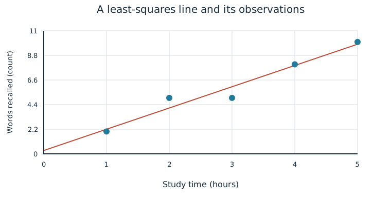
The sample means are x-bar=3 hours and y-bar=6 words. A linear regression calculation gives . Substituting the mean x=3 gives 0.3+1.9(3)=6, confirming the mean point lies on the fitted line. This is a check on the fit, not a claim that every student’s observation lies on it.
Worked Example: Squared Residuals
Predictions are 2.2,4.1,6.0,7.9,9.8 words. Residuals are −0.2,0.9,−1.0,0.1,0.2 words. Their squared sum is 0.04+0.81+1+0.01+0.04=1.90 square words. For the alternative line y-hat=2x, residuals are 0,1,−1,0,0 and their squared sum is 2.00. The LSRL has the smaller squared-error sum. It does not have to pass through an observed point or make each individual error the smallest possible.
Calculate the Fit with Technology
Enter the paired x-values and y-values in separate, matching lists or a two-column table. Select a linear regression calculation with an intercept, using study hours as x and recall counts as y. Read the slope b, y-intercept a, correlation r, and squared correlation r squared. Software sometimes prints the slope first or calls the intercept b instead of a; read the equation’s role, not just a letter label.
| Quantity | Output for these observations |
|---|---|
| Intercept a | 0.300 |
| Slope b | 1.900 |
| Correlation r | 0.974679… |
| r squared | 0.950000 |
All four numbers come from the same paired data. In simple linear regression, technology calculates the slope, the y-intercept, and correlation. Verify the sample count and variable order, then write the complete prediction equation with its contextual units. A reported coefficient without the input data and variable assignments can be impossible to interpret.
The coefficient of determination, , is the square of the correlation coefficient. It is the proportion of variation in the response variable explained by the linear relationship with the explanatory variable. Here 0.95, or 95%, of the variation in recall counts among these students is explained by the linear relationship with study hours. It is not the percentage of words each student recalls correctly and does not show that study time causes 95% of recall.
Interpret the Coefficients
The LSRL model’s coefficients are its slope b and y-intercept a, calculated from a sample of paired values. They describe the fitted sample relationship. Interpret them in the variables’ units and in context.
The slope is the predicted increase or decrease in response for a one-unit increase in the explanatory variable. In the recall example, each additional study hour is associated with a predicted increase of 1.9 recalled words under the fitted model. A negative slope would indicate a predicted decrease. The wording “predicted” matters: individual outcomes can differ, and an observational slope is not automatically an intervention effect.
The intercept is the predicted response when x=0. The example predicts 0.3 recalled words at zero study hours. But zero hours is outside the observed 1–5 hour interval, so this is an extrapolation and may have no reasonable interpretation for the studied process. An intercept can also be physically illogical even when the arithmetic is clear. For a plant-height model y-hat=−12+5x fitted to ages 4–10 weeks, the intercept predicts −12 centimeters at age zero. Height cannot be negative, so the intercept lacks a logical interpretation in that context. Both the input range and the possible response values matter.
Report and Check a Fitting Result
A useful fitting report states the data and variable assignments, the regression equation, the contextual slope and intercept, r and r squared, and any material form or range limitations. Inspect the scatterplot and residual plot to judge whether the linear form is suitable. Calculate a few predictions and signed residuals to check that outputs belong to the stated data and equation.
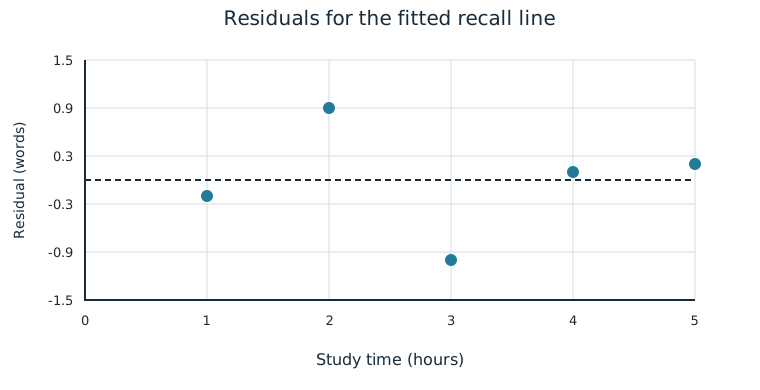
For the five recall observations, the residuals show no clear systematic curve, although the small sample limits how much can be learned about form. A large r squared does not replace the plot or prove causation. Using technology is part of the calculation; explaining what its numbers mean is part of the statistical argument.
Independent Practice
Use the information in each question to make your own calculation, representation, or argument. Explain what your result means in its setting.
Original generated practice for the Fall 2026 course.
Glossary and deeper reading · 15 refreshers
These editorial refreshers supplement the reading. Definitions and examples are added guidance; original source wording and recorded answers remain in their original context.
-
Scatterplot
A scatterplot displays paired values of two quantitative variables as points. The horizontal coordinate represents one variable and the vertical coordinate represents the other. For example, plotting hours studied against test scores helps reveal a pattern without establishing causation.
-
Least-squares regression
Least-squares regression fits a line predicting a response from an explanatory variable. The fitted line minimizes the sum of squared vertical residuals between observed and predicted responses. For example, a fitted line can predict a plant’s height from its age, within the range of observed ages.
Read more: Least-squares regression in the captured Statistics reading →
-
Residual
A residual is an observed response minus its predicted response. A positive residual places the observed point above the fitted line, while a negative residual places it below. For example, an observed height of 18 centimeters and a predicted height of 16 centimeters give a residual of 2 centimeters.
-
Mean
The mean is a measure of center often called an average. For a finite data set, the arithmetic mean is the sum of the values divided by their number; for a random variable, the mean is its probability-weighted expected value when that value exists. Means can be pulled toward extreme values and are not generally resistant. For example, the arithmetic mean of 2, 4, and 9 is 5.
-
Observation
An observation is a recorded value or set of values for an individual or occasion. The individual may be a person, object, or event rather than a human subject. For example, one plant’s measured height is an observation in a plant-growth study.
-
Regression intercept
A regression intercept is the line’s predicted response when the explanatory variable is zero. It may lack a useful contextual interpretation when zero lies outside the relevant data range. For example, an intercept predicts height at age zero even if measurements were collected only for mature plants.
Read more: Regression intercept in the captured Statistics reading →
-
Regression slope
A regression slope is the predicted change in the response for a one-unit increase in the explanatory variable. Its units are response units per explanatory-variable unit. For example, a slope of 2 centimeters per week predicts 2 additional centimeters of height for each additional week.
Read more: Regression slope in the captured Statistics reading →
-
Correlation coefficient
Pearson’s correlation coefficient measures the direction and strength of a linear relationship between two quantitative variables. It ranges from −1 to 1, and a value near 0 does not rule out a strong curved relationship. For example, points closely following a decreasing straight line have correlation near −1.
Read more: Correlation coefficient in the captured Statistics reading →
-
Coefficient of determination
The coefficient of determination is the fraction of observed response variation accounted for by a fitted regression model. In simple linear regression with an intercept, it equals the square of the correlation coefficient. For example, a value of 0.64 means that the fitted linear model accounts for 64% of the response variation in those data.
Read more: Coefficient of determination in the captured Statistics reading →
-
Response variable
A response variable records the outcome being studied. Its relationship to an explanatory variable can be investigated without assuming that the explanatory variable causes it. For example, plant height is a response when researchers compare fertilizer treatments.
Read more: Response variable in the captured Statistics reading →
-
Explanatory variable
An explanatory variable is used to predict or explain variation in a response variable. In an experiment, researchers deliberately assign values or treatments related to an explanatory variable. For example, assigned study time could be an explanatory variable when test score is the response.
Read more: Explanatory variable in the captured Statistics reading →
-
Extrapolation
Extrapolation uses a model to predict beyond the range of explanatory values used to fit it. A pattern observed within the data range may not continue outside that range. For example, extending a short-term plant-growth line far into the future may give unrealistic heights.
Read more: Extrapolation in the captured Statistics reading →
-
Residual plot
A residual plot displays prediction residuals against explanatory values or fitted responses. Curvature can suggest that a straight-line model is inappropriate, while changing spread can challenge constant-variance assumptions. For example, a U-shaped residual pattern suggests that the line misses a curved relationship.
Read more: Residual plot in the captured Statistics reading →
-
Sample
A sample is the subset of a population actually studied. How it is selected matters for the conclusions that can be drawn about the population. For example, 60 selected students may be a sample from a school’s full enrollment.
-
Causation
Causation means that changing one condition produces a change in an outcome. Association alone is insufficient because confounding and other explanations may account for the pattern. For example, a well-conducted randomized fertilizer experiment can support a causal conclusion about growth in its study setting.