4.1 Introduction to Confidence Intervals
Section Overview
- Interactive 4.1.1 - 90% Confidence Interval
- Gallery 4.1.1 - Bias and Variability
- Example 4.1.1
- Gallery 4.1.2 - 1 Samp. z-interval on Calc
- Interactive 4.1.2 - Comparing CI’s
- Pop Quiz 4.1.1
Starting with an Estimate
Hopefully by this point, you’ve begun to realize how important and necessary random sampling is in Statistics – namely that it allows us to accurately make statements about the greater population without actually having to embark on the (impossible) task of gathering data on the entire population. We’ve discussed two commonly-used statistics, the sample proportion and the sample mean , and how they help us estimate their corresponding parameters, the population proportion and the population mean . These statistics are also called point estimators, and when they take on a specific value, they are called point estimates. However, it would be foolhardy to think that a single value is equivalent to the value of the actual parameter. Thus, we use confidence intervals, which allow the parameter to fall into a range of possible values. They are written in the form:
where the margin of error is composed of the critical value and the standard error of the statistic, giving us the final form of:
The standard error of the point estimate depends on whether we’re dealing with the sample proportion or the sample mean, but the critical value of a confidence interval depends on the confidence level . A confidence level can take any value, but the most common are at the 90%, 95%, and 99% level. For the sample proportion, the critical values that correspond to these confidence levels are shown in the following table:
| Confidence Level | 90% | 95% | 99% |
|---|---|---|---|
| Critical Value | 1.645 | 1.960 | 2.576 |
The critical values for a sample proportion are similar to the z-values taken from the z-table, except that these values are not derived from the data set, and as such are denoted by and . Our confidence interval for the sample proportion, or our one-sample z interval becomes:
where:
- = sample proportion
- = sample size
- = critical z-value of confidence interval
We will discuss the critical values and the confidence interval for the sample mean in a later section, as these depend on the t-distribution.
Using Confidence Intervals Wisely
Ever wonder why we don’t always just use 99% (or even 100%) confidence intervals? It’s because you have to pay a price for that extra confidence: the larger you make your confidence interval, the larger your margin of error will be. Now you might be asking what it actually means to be 99% confident. It means that 99% of our intervals will contain the true value of the parameter. It does NOT mean that there is a 99% chance an interval will contain the true value of the parameter. The confidence interval either contains the true value or it doesn’t. All of this holds true for every other confidence level. This concept is demonstrated in Interactive 4.1.1.
Before constructing a confidence interval, we also want to make sure the following conditions are met:
- Random – The data we use comes from a random sample or randomized experiment.
- Normal – For the sampling distribution of the sample proportion, we want to make sure that there are at least 10 successes and 10 failures in the sample, or and . The sampling distribution of the sample mean will be approximately Normal if as ensured by the Central Limit Theorem.
- Independent – The observations within the sample or group should be independent of one another. The formulas we use for the standard deviation assume that we are sampling with replacement which would ensure that the sample mean and proportion would not be affected by an ever-decreasing population pool. More often, however, we are sampling without replacement so we want to make sure that the population is at least 10 times as large as the sample, or .
Interactive 4.1.1 90% Confidence Intervals
Properties of Point Estimators
Although we can easily take a random sample and come up with a statistic/point estimator, we look at two properties:
- Bias – When we previously looked at bias, we defined it as systematically favoring a certain outcome. We call a point estimator unbiased if the mean of its sampling distribution is equal to the actual value of the parameter (yes, this still applies to the mean of the sampling distribution of the sample proportion .) How do we know if a point estimator is unbiased if we don’t even know the actual value of the parameter, however? We can often prove it mathematically, but doing so is outside the scope of this text. Just know that you won’t have to worry about either the sample proportion or the sample mean, because they are known to be unbiased point estimators.
- Variability – A point estimator can be unbiased, but still have a lot of variability if the sample size is too small. In Gallery 3.6.1, when we changed the sample size from (1st slide) to (3rd slide) to (4th slide), notice how the possible values the sample proportion took also shrank in size. In this case, choosing the sample size of would ensure that the point estimator will have the least amount of variability.
Gallery 4.1.1 shows the different combinations of bias and variability we can have when getting our point estimate.
Gallery 4.1.1 Bias and Variability of Point Estimators
Frame 1 of 4
High bias and high variability Open full-size image S0338Frame 2 of 4
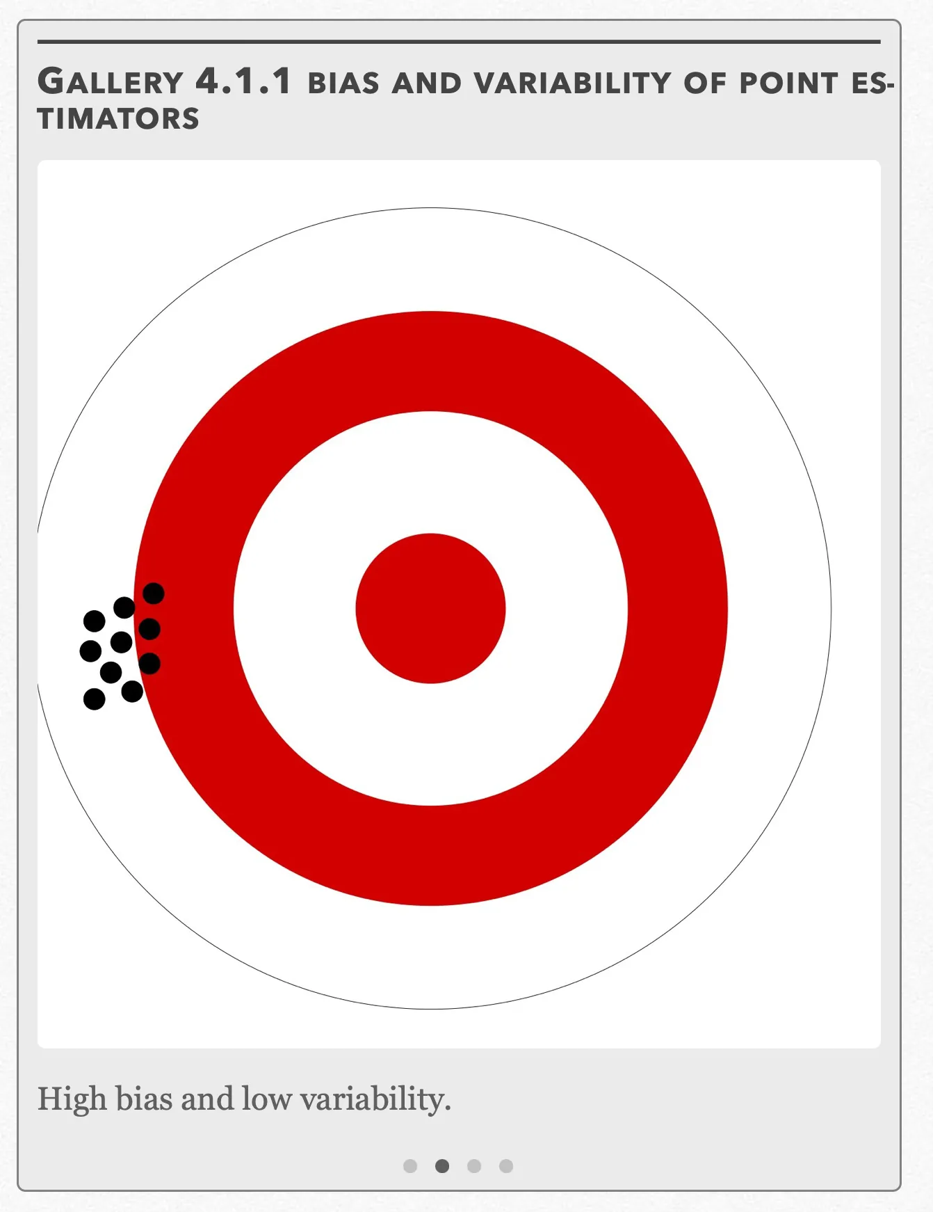
High bias and low variability. Open full-size image S0339Frame 3 of 4
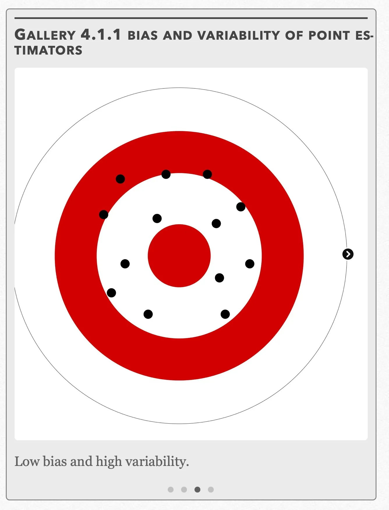
Low bias and high variability. Open full-size image S0340Frame 4 of 4
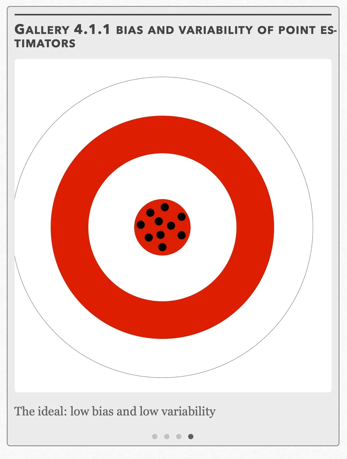
The ideal: low bias and low variability Open full-size image S0341
Capture provenance
Filename capture times, with no recorded timezone. Frames above follow the original gallery positions.
- · S0338 · displayed frame 1
Screenshot 2026-10-05 at 4.00.42 PM.png - · S0339 · displayed frame 2
Screenshot 2026-10-05 at 4.00.49 PM.png - · S0340 · displayed frame 3
Screenshot 2026-10-05 at 4.00.54 PM.png - · S0341 · displayed frame 4
Screenshot 2026-10-05 at 4.00.59 PM.png
Example 4.1.1
Will it Mend?, a large company that fixes all manner of objects large and small, wants to conduct a survey that will help them gauge general customer satisfaction. The survey will randomly select customers.
(a) Find how large a sample is needed, if the company wants the estimate to be within a 2.5% margin of error at a 95% confidence level.
(b) After conducting the survey and receiving the results, the company finds that 87% of customers are satisfied with their service. Find the confidence interval.
(c) Find the new confidence interval if the confidence level in (b) was changed to 90%.
(d) Find the new confidence interval if the sample size in (b) is changed to (assume that the sample proportion does not change.)
Example 4.1.1 — recorded source answer
(a) If we want our margin of error to be within 2.5%, we have:
When is unknown, it is common to use the value of 0.5, getting us:
When we isolate the and square both sides we get:
Will it Mend? needs a sample size of 1537 people to ensure that the margin of error is at most 2.5%. Note that even if our final result was something like 1536.15 instead, we would still say that we needed a sample of size 1537 because it better ensures that the sample is within the margin of error.
(b) First, we want to check our three conditions:
Random – It was mentioned that the survey will be composed of randomly selected customers, so this condition checks out.
Normal - and , so this condition checks out, as well.
Independent – It was mentioned that the company was large so we can assume that there at least customers that have used Will it Mend?’s services.
Using the formula for our one-sample z interval, we get:
We are 95% confident that between 85.3% to 88.7% captures the true proportion of customers who are satisfied.
See Gallery 4.1.2 for how to perform these steps on your calculator.
(c) If the confidence level was changed to 90%, the critical value would change, making our confidence interval:
We are 90% confident that between 85.6% to 88.4% of customers are satisfied with the service.
See Gallery 4.1.2 for how to perform these steps on your calculator.
(d) If the confidence interval had a new sample size of , our new confidence interval would be:
We are 95% confident that the interval from 0.8492 to 0.8908 captures the true proportion of customers who are satisfied.
See Gallery 4.1.2 for how to perform these steps on your calculator.
Interactive 4.1.2 compares the confidence
Gallery 4.1.2 Example 4.1.1 (One-Sample z Interval on TI 83/84)
Frame 1 of 7
Press the STAT button, go to TESTS, choose “1-PropZInt” and press ENTER. Open full-size image S0344Frame 2 of 7
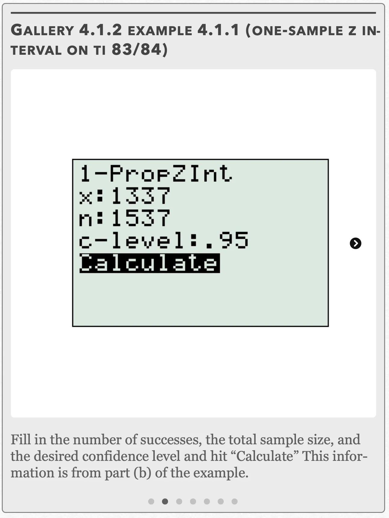
Fill in the number of successes, the total sample size, and the desired confidence level and hit “Calculate” This information is from part (b) of the example. Open full-size image S0345Frame 3 of 7
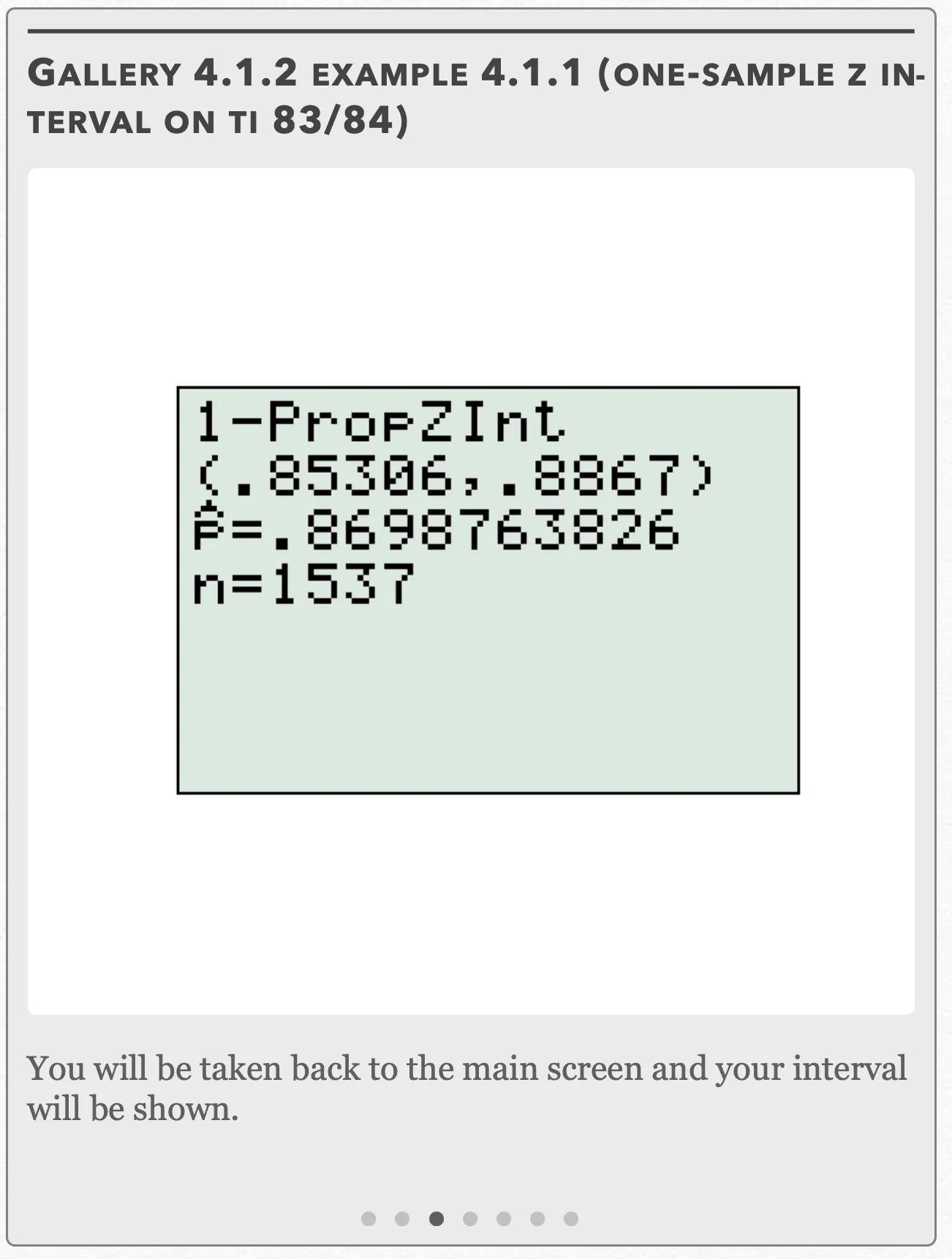
You will be taken back to the main screen and your interval will be shown. Open full-size image S0346Frame 4 of 7
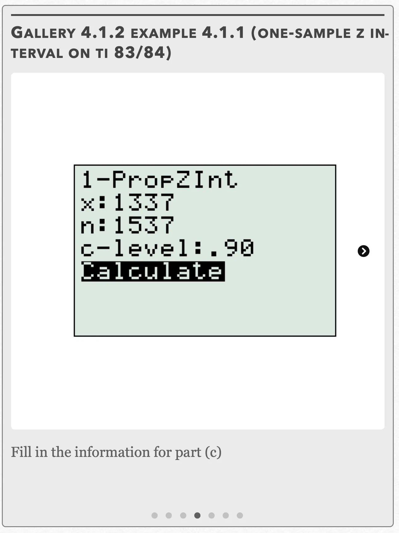
Fill in the information for part (c) Open full-size image S0347Frame 5 of 7
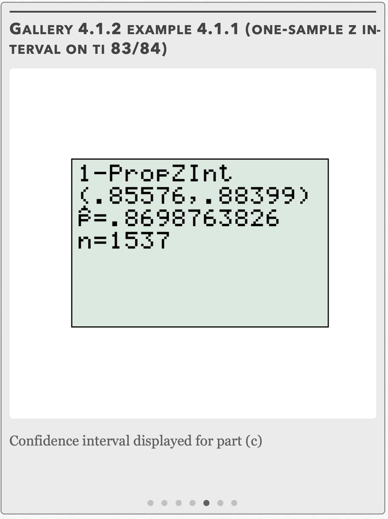
Confidence interval displayed for part (c) Open full-size image S0348Frame 6 of 7
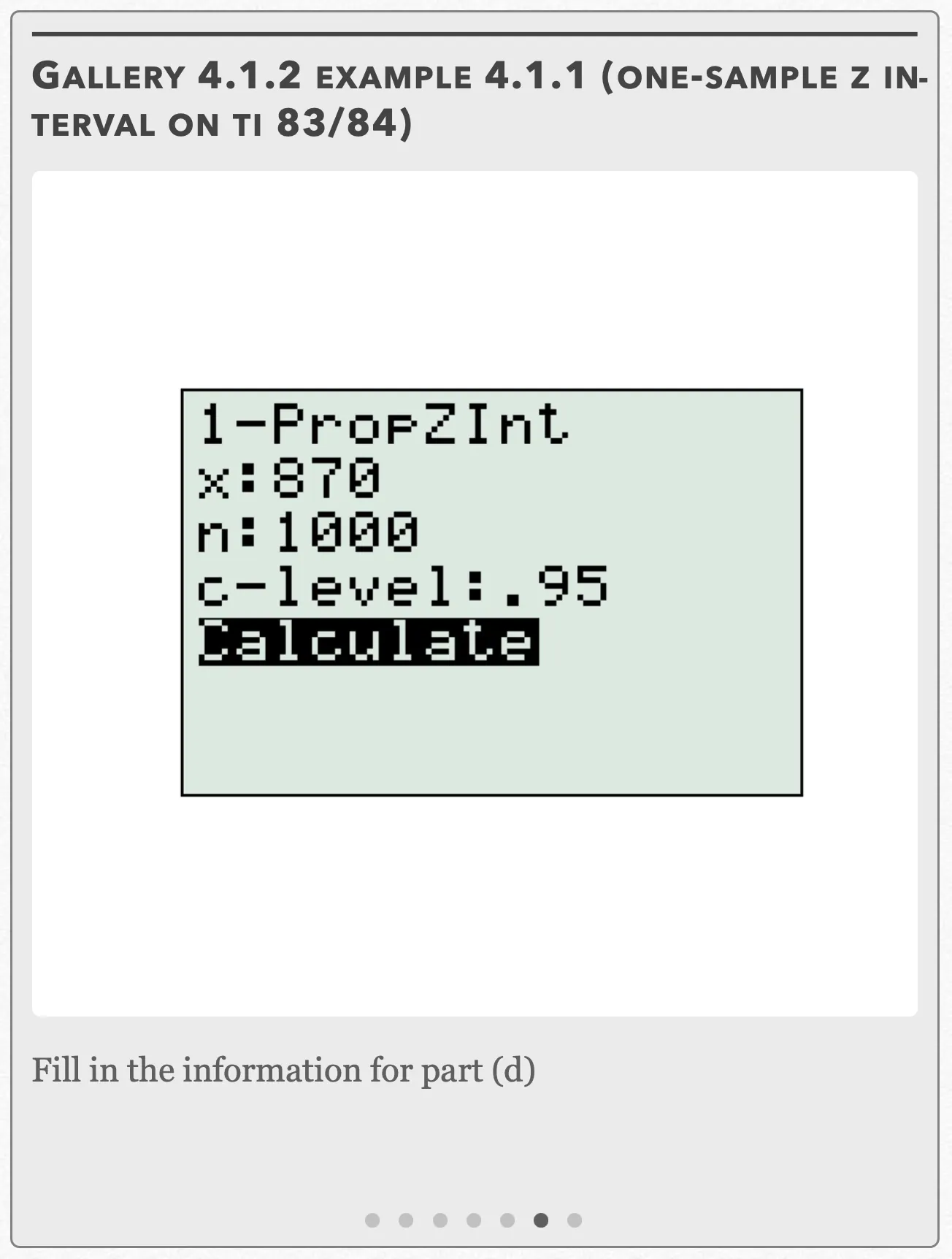
Fill in the information for part (d) Open full-size image S0349Frame 7 of 7
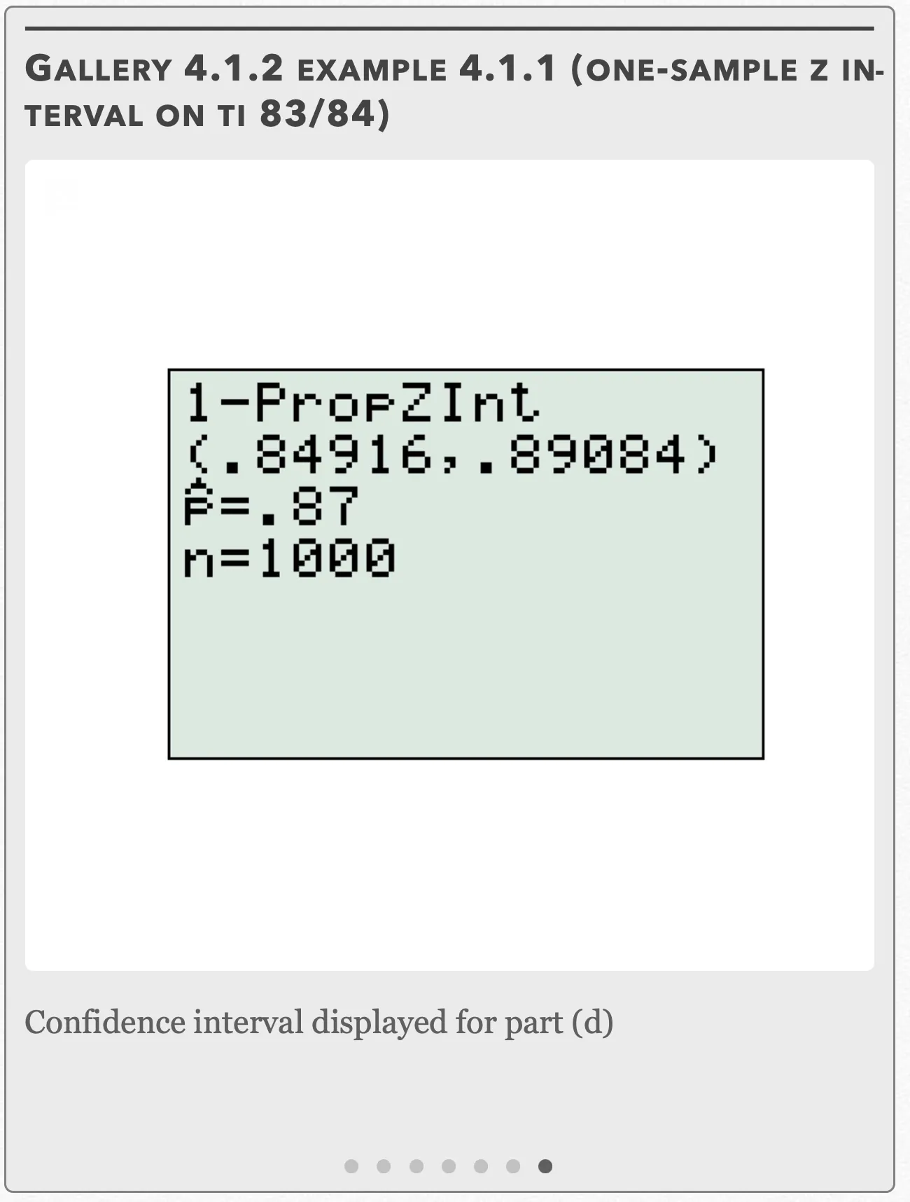
Confidence interval displayed for part (d) Open full-size image S0350
Capture provenance
Filename capture times, with no recorded timezone. Frames above follow the original gallery positions.
- · S0344 · displayed frame 1
Screenshot 2026-10-05 at 4.01.04 PM.png - · S0345 · displayed frame 2
Screenshot 2026-10-05 at 4.01.10 PM.png - · S0346 · displayed frame 3
Screenshot 2026-10-05 at 4.01.15 PM.png - · S0347 · displayed frame 4
Screenshot 2026-10-05 at 4.01.20 PM.png - · S0348 · displayed frame 5
Screenshot 2026-10-05 at 4.01.25 PM.png - · S0349 · displayed frame 6
Screenshot 2026-10-05 at 4.01.30 PM.png - · S0350 · displayed frame 7
Screenshot 2026-10-05 at 4.01.35 PM.png
Interactive 4.1.2 Example 4.1.1 (Comparing Confidence Intervals)
Pop Quiz 4.1.1
Glossary and deeper reading · 23 refreshers
These editorial refreshers supplement the reading. Definitions and examples are added guidance; original source wording and recorded answers remain in their original context.
-
Random sampling
Random sampling uses a specified chance process to select individuals from a population. It supports population inference when the sampling frame and data collection are appropriate, but does not guarantee perfect balance or eliminate every source of bias. For example, a random-number generator can select student identifiers from an enrollment list.
Read more: Random sampling in the captured Statistics reading →
-
Population
A population is the full set of individuals or measurements a study aims to describe. It must be defined clearly before deciding whether a sample supports generalization. For example, all students enrolled in a particular school this year form a population.
-
Margin of error
A margin of error is the amount added to and subtracted from a point estimate in a symmetric confidence interval. In the procedures here it combines a critical value with an estimated standard error and addresses modeled sampling variability. For example, an estimate of 40% with a margin of 3 percentage points gives an interval from 37% to 43%.
-
Critical value
A critical value is a cutoff from a reference distribution chosen for a confidence level or testing rule. The relevant distribution, degrees of freedom, and one-sided or two-sided procedure determine the cutoff. For example, a symmetric 95% Normal interval uses a cutoff near 1.96 standard-error units.
-
Standard error
A standard error describes the standard deviation of a statistic’s sampling distribution, usually estimated from data. It measures uncertainty in an estimate rather than the spread of individual observations. For example, the estimated standard error of a sample mean is the sample standard deviation divided by the square root of the sample size.
-
Point estimate
A point estimate is the specific numerical value obtained from an estimator for the observed sample. It gives one estimate without expressing uncertainty by itself. For example, a sample mean of 14 minutes is a point estimate of the population’s mean travel time.
-
Sample proportion
A sample proportion is the number of sampled individuals with a specified characteristic divided by the sample size. It is commonly written p-hat and estimates the corresponding population proportion. For example, 18 walkers among 60 sampled students give a sample proportion of 0.30.
Read more: Sample proportion in the captured Statistics reading →
-
Z-score
A z-score expresses a value’s distance from its distribution’s mean in standard-deviation units. It is found by subtracting the mean from the value and dividing by the standard deviation. For example, a z-score of −1.5 places the value 1.5 standard deviations below the mean.
-
Sample
A sample is the subset of a population actually studied. How it is selected matters for the conclusions that can be drawn about the population. For example, 60 selected students may be a sample from a school’s full enrollment.
-
Mean
The mean is a measure of center often called an average. For a finite data set, the arithmetic mean is the sum of the values divided by their number; for a random variable, the mean is its probability-weighted expected value when that value exists. Means can be pulled toward extreme values and are not generally resistant. For example, the arithmetic mean of 2, 4, and 9 is 5.
-
Student’s t-distribution
A Student’s t-distribution is a symmetric reference distribution with heavier tails than the standard Normal distribution. Its shape depends on degrees of freedom and approaches the standard Normal shape as those degrees of freedom grow. For example, inference about a Normal population mean with an unknown standard deviation uses a t reference with one fewer degree of freedom than the sample size.
Read more: Student’s t-distribution in the captured Statistics reading →
-
Population parameter
A population parameter is a numerical feature of the population or probability model being studied. It is fixed for that defined population, although its value may be unknown. For example, the true proportion of all enrolled students who walk to school is a parameter.
Read more: Population parameter in the captured Statistics reading →
-
Confidence level
A confidence level is the long-run fraction of intervals from a procedure that capture the true parameter under its assumptions. Holding the data and procedure fixed, increasing the confidence level generally widens the interval. For example, a 99% interval is usually wider than a 90% interval calculated from the same sample.
-
Experiment
An experiment deliberately imposes treatments and measures responses. Random assignment, comparison, and replication help distinguish treatment effects from other variation. For example, assigning plants to fertilizer treatments is an experiment.
-
Sampling distribution of a sample proportion
The sampling distribution of a sample proportion describes proportions obtained from repeated samples of a fixed size. A Normal approximation requires an appropriate design and sufficiently large expected success and failure counts. For example, larger independent samples usually give sample proportions that vary less around the population proportion.
Read more: Sampling distribution of a sample proportion in the captured Statistics reading →
-
Sampling distribution of a sample mean
The sampling distribution of a sample mean describes averages from repeated samples of a fixed size. For independent identically distributed observations with finite variance, its mean is the population mean and its standard deviation is the population standard deviation divided by the square root of the sample size. For example, averages from samples of 100 measurements vary less than averages from samples of 25.
Read more: Sampling distribution of a sample mean in the captured Statistics reading →
-
Statistical independence
Statistical independence means that learning one outcome does not change the probability distribution of another. For two events, it implies that the probability of both occurring equals the product of their probabilities. For example, independent draws with replacement keep the second draw’s color probabilities unchanged by the first.
Read more: Statistical independence in the captured Statistics reading →
-
Observation
An observation is a recorded value or set of values for an individual or occasion. The individual may be a person, object, or event rather than a human subject. For example, one plant’s measured height is an observation in a plant-growth study.
-
Sample statistic
A statistic is a numerical summary calculated from sample data. Its value can change when a different sample is selected from the same population. For example, the proportion of walkers among 60 sampled students is a statistic.
Read more: Sample statistic in the captured Statistics reading →
-
Point estimator
A point estimator is a rule that uses sample data to produce one estimate of a population parameter. The rule has a sampling distribution before the sample is observed. For example, computing the sample mean is a point estimator of the population mean.
-
Statistical bias
Statistical bias is a systematic tendency to favor some outcomes or miss a target value. For an estimator, bias is its long-run average estimate minus the parameter it estimates. For example, a survey that consistently misses evening workers may systematically misrepresent commuting patterns.
Read more: Statistical bias in the captured Statistics reading →
-
Unbiased estimator
An unbiased estimator has a sampling-distribution mean equal to the parameter being estimated. Individual estimates can still differ substantially from the parameter, so unbiased does not mean perfectly accurate. For example, a properly sampled mean can be unbiased even when small samples produce highly variable estimates.
-
Sampling variability
Sampling variability describes how an estimate changes across repeated samples drawn with the same design. Larger suitable random samples generally reduce this variability, without automatically correcting systematic bias. For example, means from samples of 100 students usually vary less than means from samples of 10 students.