4.6 Intervals and Tests for Two Means
Section Overview
- Gallery 4.6.1 — 1 & 2 sided tests for 2 Means
- Example 4.6.1
- Gallery 4.6.2 — 2 Samp. t-test on Calc
- Gallery 4.6.3 — 2 Samp. t-interval on Calc
- Interactive 4.6.1 — Example 4.6.1
- Pop Quiz 4.6.1
Similarities with Other Sample Statistics
By now, you’ve probably noticed a pattern with how confidence intervals and significance tests are structured for the various sample statistics. The difference between two sample means x̄₁ − x̄₂ shares some similarities with them.
Conditions for Two-Sample Statistics: The conditions needed to perform the two-sample t test or the two-sample t interval are very similar to the conditions needed to perform the two-sample z test or the two-sample z interval. This is because the Random, Normal, and Independent conditions had to apply to both samples that made up the two-sample statistic as shown back in Chapter 4.4.
The Normal Condition: The sample size conditions that must be met to perform one-sample t-procedures also apply to our two-sample t procedures. See Chapter 4.5 for more details.
One and Two-Sided Tests: The one and two-sided tests for the difference between sample means are performed the same way as one and two-sided tests for the sample mean. See Gallery 4.6.1 for more details.
Paired Procedures: Back when we went over matched pairs design, we mentioned how either both treatments were either randomly assigned to one experimental unit or how each treatment was assigned to two similar experimental units (usually the former.) If we are ever asked to perform t-procedures on this type of experimental design, then we use the one-sample t procedures, where the mean being tested is the difference between the means for each treatment. This is because two-sample t-procedures can only be used when the treatment groups are independent.
Significance Tests for Two Means
When performing significance tests for the difference between two sample means x̄₁ − x̄₂, we use the two-sample t test to find the t-statistic:
where x̄₁ − x̄₂ = difference between sample mean 1 and sample mean 2; μ₁ − μ₂ = difference between population mean 1 and population mean 2; s₁ = standard deviation of sample 1; s₂ = standard deviation of sample 2; n₁ = size of sample 1; n₂ = size of sample 2.
Our null hypothesis is: .
We also have our three possible alternative hypotheses, where:
See Gallery 4.6.1 for a visualization of one and two-sided tests.
Confidence Intervals for Two Means
The two-sample t interval for the difference between two sample means x̄₁ − x̄₂ is:
where x̄₁ − x̄₂ = difference between sample mean 1 and sample mean 2; s₁ = standard deviation of sample 1; s₂ = standard deviation of sample 2; n₁ = size of sample 1; n₂ = size of sample 2; t* = critical t-value.
Gallery 4.6.1 One and two-sided significance tests for two means
Frame 1 of 3
A possible one-sided test where the area to the right of the t-statistic is the p-value. Open full-size image S0439Frame 2 of 3
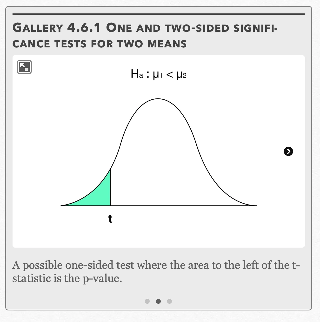
A possible one-sided test where the area to the left of the t-statistic is the p-value. Open full-size image S0440Frame 3 of 3
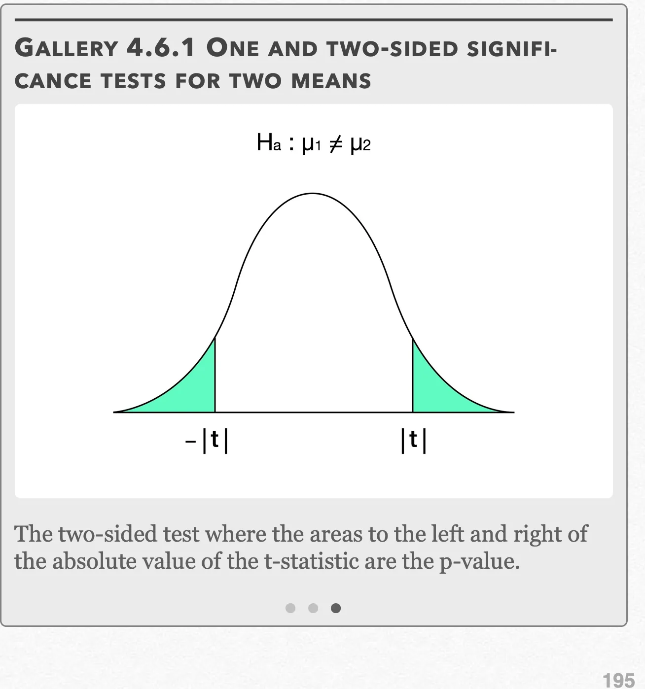
The two-sided test where the areas to the left and right of the absolute value of the t-statistic are the p-value. Open full-size image S0441
Capture provenance
Filename capture times, with no recorded timezone. Frames above follow the original gallery positions.
- · S0439 · displayed frame 1
Screenshot 2026-10-05 at 4.05.33 PM.png - · S0440 · displayed frame 2
Screenshot 2026-10-05 at 4.05.37 PM.png - · S0441 · displayed frame 3
Screenshot 2026-10-05 at 4.05.41 PM.png
Example 4.6.1
Recall in Chapter 2.2 that a drug company wanted to see if their pill, called IQuick, could actually enhance mental acuity. 111 people were randomly selected for the study, with 56 subjects randomly assigned to take IQuick for four weeks and 55 subjects randomly assigned to take a placebo for four weeks. At the end of the study, a comprehensive test is given to the subjects, and based on an algorithm, the subjects are given a (non-integer) score ranging from 0 to 10 points. The IQuick group had an average score of x̄ = 8.78 points with a standard deviation of sₓ = 0.44 points, while the placebo group had an average score of x̄ = 8.59 points with a standard deviation of sₓ = 0.63 points.
(a) Is there sufficient evidence at the α = 0.01 level to suggest that the IQuick pill may increase mental acuity more than a placebo?
(b) Construct a confidence interval consistent with the results in (a).
Example 4.6.1 — solution (a)
(a) First, we want to check our three conditions:
Random — The 111 subjects were randomly assigned to the two treatments, so this condition checks out.
Normal — Since n = 56 > 30, and n = 55 > 30 we are safe to use the t-procedures, even if the distribution is non-Normal.
Independent — Due to the random assignment, the two treatment groups can be seen as independent. Individuals within groups can also be seen as independent from one another; the change in one subject’s mental acuity gives us no information about another subject’s response.
Since we want to know if the results from the IQuick pill are greater than the results from the placebo, we use a one-sided test:
Using the formula for the two-sample t test to calculate the t-statistic, we get:
Gallery 4.6.2 Example 4.6.1 (two-sample t test on TI 83/84)
Frame 1 of 3
Press the STAT button, go to TESTS, choose “2-SampTTest” and press ENTER Open full-size image S0443Frame 2 of 3
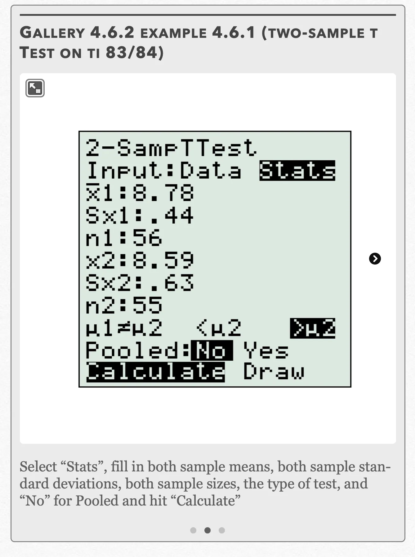
Select “Stats”, fill in both sample means, both sample standard deviations, both sample sizes, the type of test, and “No” for Pooled and hit “Calculate” Open full-size image S0444Frame 3 of 3
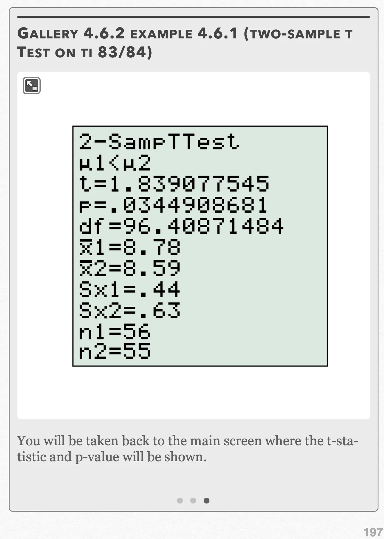
You will be taken back to the main screen where the t-statistic and p-value will be shown. Open full-size image S0445
Capture provenance
Filename capture times, with no recorded timezone. Frames above follow the original gallery positions.
- · S0443 · displayed frame 1
Screenshot 2026-10-05 at 4.05.44 PM.png - · S0444 · displayed frame 2
Screenshot 2026-10-05 at 4.05.50 PM.png - · S0445 · displayed frame 3
Screenshot 2026-10-05 at 4.05.54 PM.png
Refer to Gallery 4.6.2 for how to perform these steps on your calculator.
We want to compare the t-statistic to the critical t-value. To find the critical t-value, we need the upper tail probability and the degrees of freedom. We have a one-sided test at α = 0.01. Additionally, since our sample sizes are different, we’ll use the smaller of our degrees of freedom, 55 − 1 = 54. Looking at the t-table, however, we see that there is no entry for df = 54, so we use the more conservative df = 50. With these two pieces of information, we get t* = 2.403 from the t-table.
Since t < t*, or 1.839 < 2.403, we fail to reject the null hypothesis. We do not have enough evidence to say that the IQuick pill helps improve mental acuity any more than a placebo.
Additionally, if we use our calculator, we see that our p-value is 0.034, which is smaller than the significance level at α = 0.01.
Example 4.6.1 — solution (b)
(b) We do not need to prove the Random, Normal, or Independent conditions again, since the conditions apply to all t-procedures.
Since confidence intervals are inherently two-sided and our significance test was one-sided, we want to use a confidence level at 98%. We already found this value to be t* = 2.403 in part (a).
Using the formula for the two-sample t-interval, we get:
Gallery 4.6.3 Example 4.6.1 (two-sample t interval on TI 83/84)
Frame 1 of 3
Press the STAT button, go to TESTS, choose “2-SampTInt” and press ENTER Open full-size image S0447Frame 2 of 3
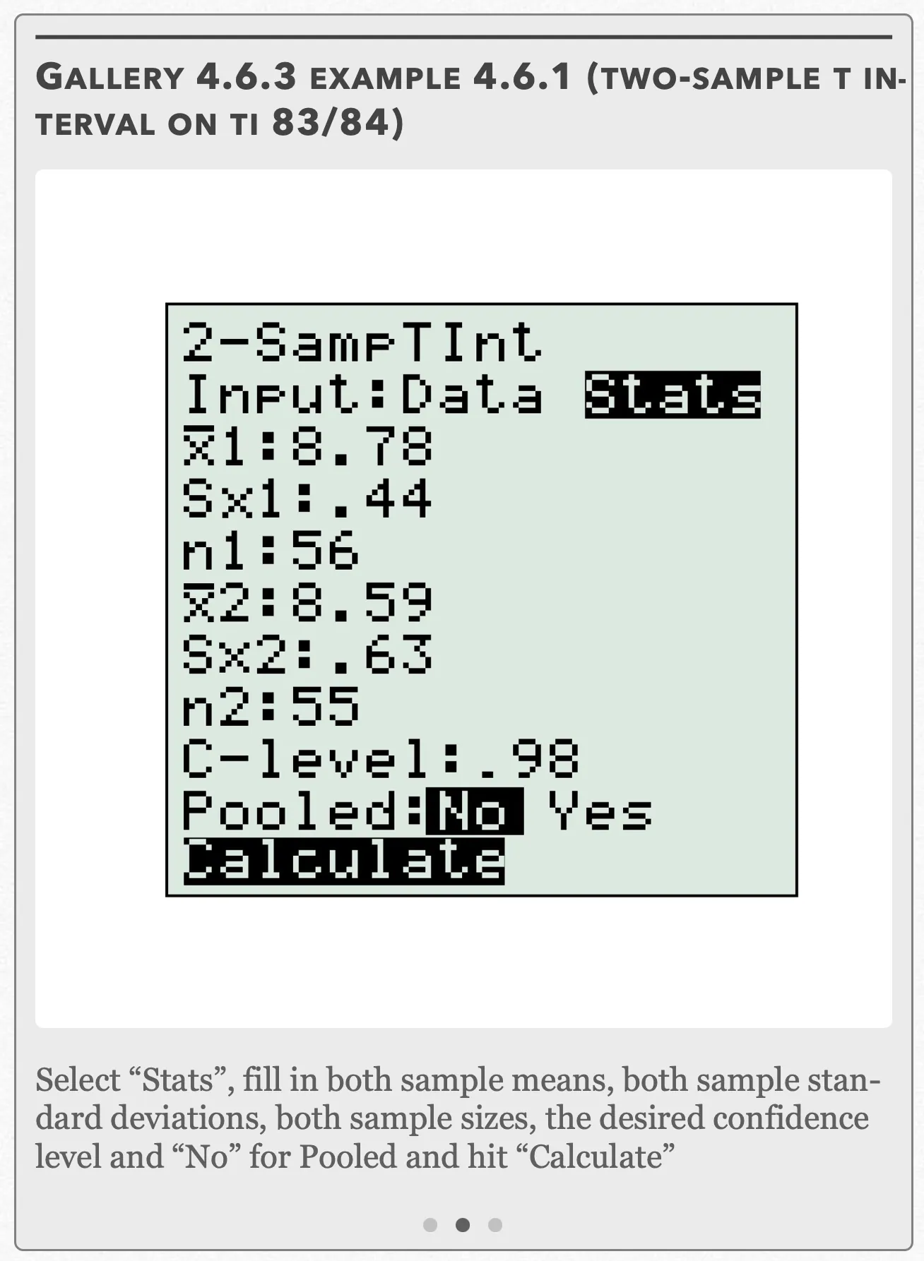
Select “Stats”, fill in both sample means, both sample standard deviations, both sample sizes, the desired confidence level and “No” for Pooled and hit “Calculate” Open full-size image S0448Frame 3 of 3
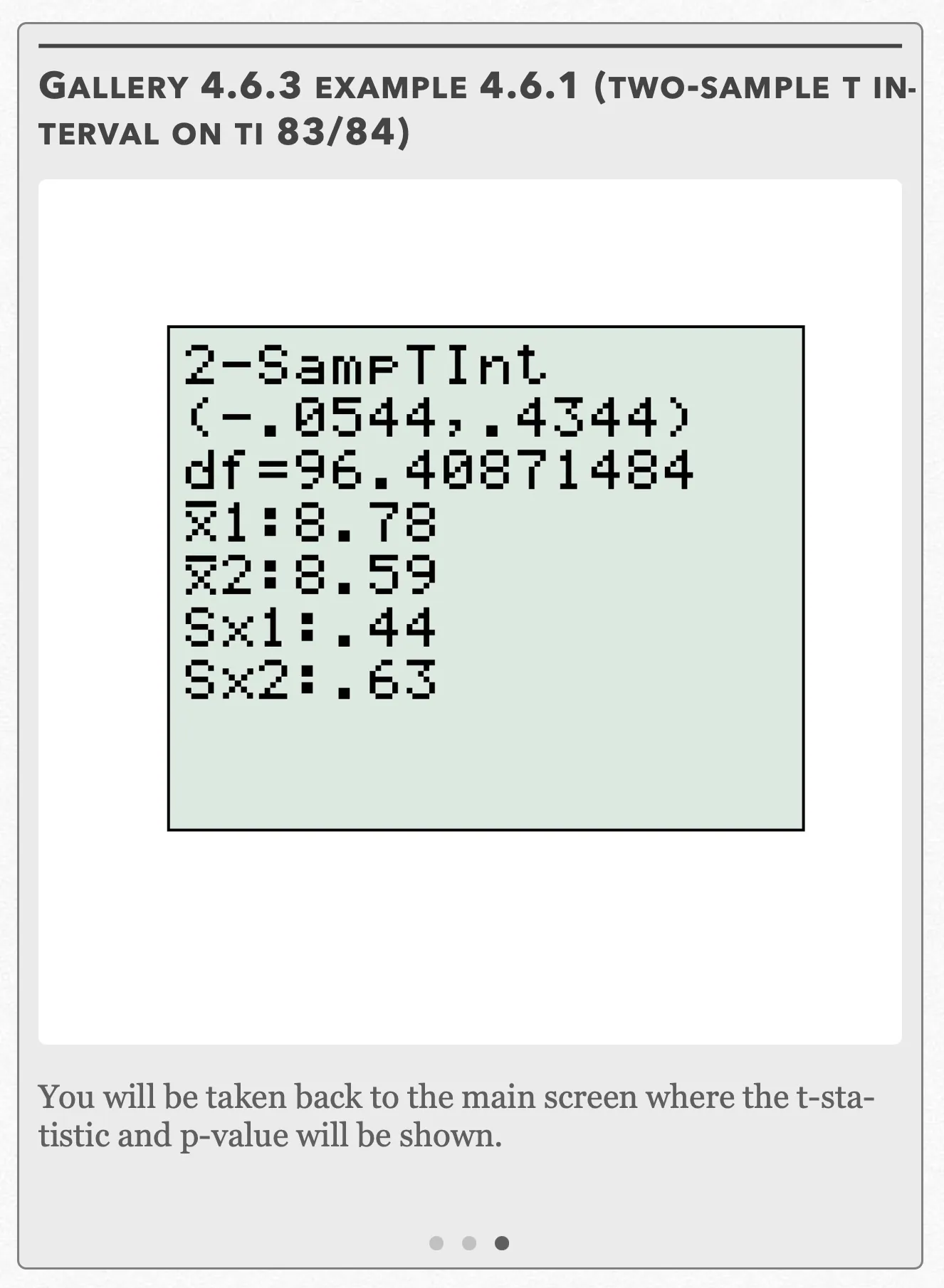
You will be taken back to the main screen where the t-statistic and p-value will be shown. Open full-size image S0449
Capture provenance
Filename capture times, with no recorded timezone. Frames above follow the original gallery positions.
- · S0447 · displayed frame 1
Screenshot 2026-10-05 at 4.05.58 PM.png - · S0448 · displayed frame 2
Screenshot 2026-10-05 at 4.06.03 PM.png - · S0449 · displayed frame 3
Screenshot 2026-10-05 at 4.06.07 PM.png
Refer to Gallery 4.6.3 for how to perform these steps on your calculator.
We are 98% confident that the mean score for the IQuick group is between 0.05 points lower and 0.43 points higher than the mean score for the placebo group. Since 0 is included in this interval (meaning that there is no difference in scores between the two groups), this agrees with the results from the significance test in (a) where it states that we lack the evidence to say if the IQuick pill actually improves mental acuity more than a placebo.
Interactive 4.6.1 Example 4.6.1
Pop Quiz 4.6.1
Glossary and deeper reading · 15 refreshers
These editorial refreshers supplement the reading. Definitions and examples are added guidance; original source wording and recorded answers remain in their original context.
-
Confidence interval
A confidence interval is a data-based range produced by a method with a specified long-run coverage rate for a population parameter. For a fixed population, the calculated interval either contains the parameter or it does not; the confidence level describes the method over repeated samples. For example, a 95% method captures the true parameter in about 95% of repeated intervals when its assumptions hold.
Read more: Confidence interval in the captured Statistics reading →
-
Significance test
A significance test assesses how compatible observed data are with a specified null model. It compares a test statistic or p-value with a decision rule chosen for the study. For example, a test can assess whether a sample provides evidence that a population walking proportion differs from a stated value.
Read more: Significance test in the captured Statistics reading →
-
Sample statistic
A statistic is a numerical summary calculated from sample data. Its value can change when a different sample is selected from the same population. For example, the proportion of walkers among 60 sampled students is a statistic.
Read more: Sample statistic in the captured Statistics reading →
-
Two-sample z procedure for proportions
A two-sample z procedure uses a Normal approximation to compare two population proportions from independent groups. The equality test pools proportions for its null standard error, while the usual confidence interval uses separate sample proportions. For example, it can compare preference proportions from independently sampled students in two schools when its conditions hold.
Read more: Two-sample z procedure for proportions in the captured Statistics reading →
-
Sample
A sample is the subset of a population actually studied. How it is selected matters for the conclusions that can be drawn about the population. For example, 60 selected students may be a sample from a school’s full enrollment.
-
One-sample t procedure
A one-sample t procedure makes inference about a population mean using the sample mean and sample standard deviation. It requires an appropriate study design and a sufficiently suitable distribution of the mean, with particular care for small samples, strong skewness, and outliers. For example, a random sample of travel times can estimate a population mean when the assumptions are defensible.
Read more: One-sample t procedure in the captured Statistics reading →
-
Difference between sample means
A difference between sample means compares two groups’ observed averages. Inference must reflect whether the samples are independent or paired rather than treating every comparison the same way. For example, two independently sampled classes’ mean travel times can estimate a difference between their population means.
Read more: Difference between sample means in the captured Statistics reading →
-
Mean
The mean is a measure of center often called an average. For a finite data set, the arithmetic mean is the sum of the values divided by their number; for a random variable, the mean is its probability-weighted expected value when that value exists. Means can be pulled toward extreme values and are not generally resistant. For example, the arithmetic mean of 2, 4, and 9 is 5.
-
Matched pairs design
A matched pairs design compares two treatments within matched units or within the same unit. Assignment within pairs or treatment order is randomized when the design permits, and analysis uses the pairwise differences. For example, two shoe designs can be compared on the same person with their left-right assignment randomized.
Read more: Matched pairs design in the captured Statistics reading →
-
Treatment
A treatment is a specific condition imposed on an experimental unit. In a multifactor experiment, a treatment is a combination of factor levels. For example, low fertilizer with eight hours of light is one treatment combination.
-
Test statistic
A test statistic summarizes how the sample departs from the null model. Its reference distribution under the null supplies the probabilities used in testing. For example, a z-statistic expresses a sample proportion’s difference from a hypothesized proportion in null-model standard-error units.
Read more: Test statistic in the captured Statistics reading →
-
Standard deviation
Standard deviation measures spread around the mean using squared deviations and a square root. A sample standard deviation uses the sum of squared deviations divided by one less than the sample size before taking the square root. For example, a larger standard deviation of travel times indicates greater variability, in the original time units.
Read more: Standard deviation in the captured Statistics reading →
-
Null hypothesis
A null hypothesis specifies the reference claim or model used to calculate a test’s probabilities. It commonly states no population difference or a particular parameter value. For example, a null hypothesis can state that the population mean travel time equals 15 minutes.
Read more: Null hypothesis in the captured Statistics reading →
-
Alternative hypothesis
An alternative hypothesis specifies the population difference or direction for which a test seeks evidence. It should be chosen from the research question before inspecting results. For example, an alternative can state that the population mean travel time is greater than 15 minutes.
Read more: Alternative hypothesis in the captured Statistics reading →
-
Critical value
A critical value is a cutoff from a reference distribution chosen for a confidence level or testing rule. The relevant distribution, degrees of freedom, and one-sided or two-sided procedure determine the cutoff. For example, a symmetric 95% Normal interval uses a cutoff near 1.96 standard-error units.
Read more: Critical value in the captured Statistics reading →