Describe a Quantitative Distribution in Context — Worked Solutions
Worked Solutions
Compare your reasoning with the worked solutions after attempting the questions. A different valid representation or explanation can earn credit when it satisfies the stated criteria.
Original generated practice for the Fall 2026 course. Return to the lesson and independent checks.
Describe community-room setup times: worked answer
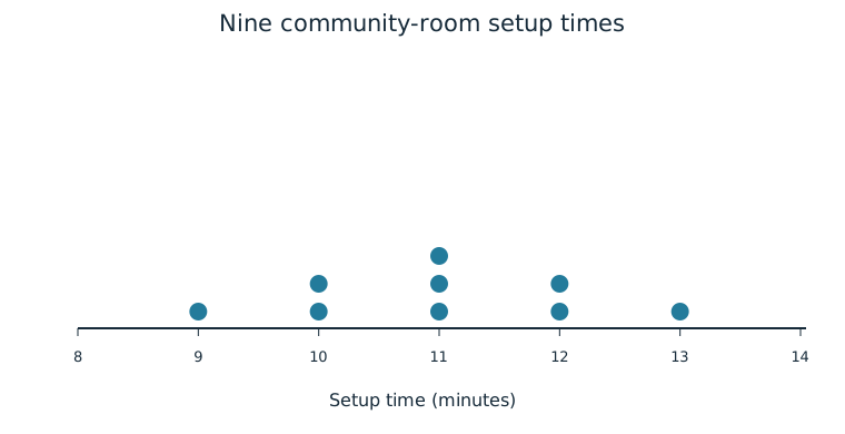
Nine measured setup times for a community room, in minutes, are 9,10,10,11,11,11,12,12,13. The dotplot represents every observation.
Part a
Describe shape, approximate center, and observed spread in context. Use specific matching values and their frequencies on opposite sides of the center to justify your shape description, and identify any main peak.
These community-room setup times are symmetric and unimodal around 11 minutes, with observed times from 9 to 13 minutes (a range of 4 minutes). There is one observation at both 9 and 13, two at both 10 and 12, and three at 11. Those matching counts at equal distances from 11 justify mirrored halves and a single main peak. This describes the nine measured times; it does not prove every future setup distribution has the same shape.
| Evidence for credit | Points |
|---|---|
| Describes the setup-time shape as symmetric and unimodal, center about 11 minutes and observed 9–13-minute spread with units. | 1 |
| Justifies symmetry with matched 9/13 and 10/12 frequencies and identifies the three observations at 11 as the single main peak. | 1 |
Name the longer tail: worked answer
Part a
Describe each skew direction and explain using the tail toward larger or smaller values.
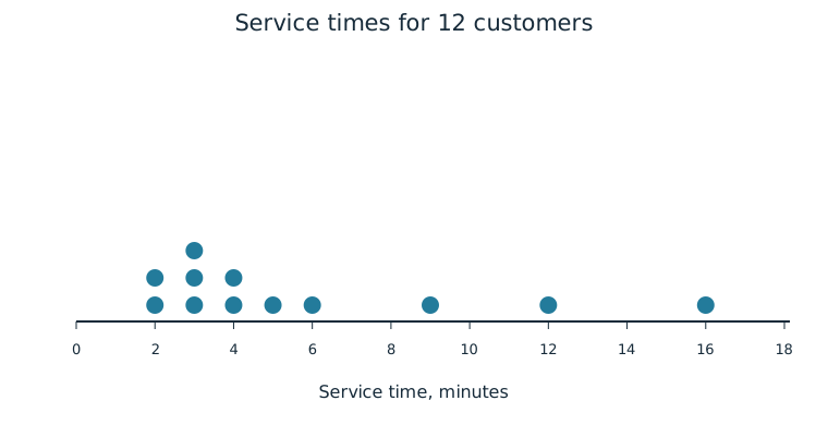
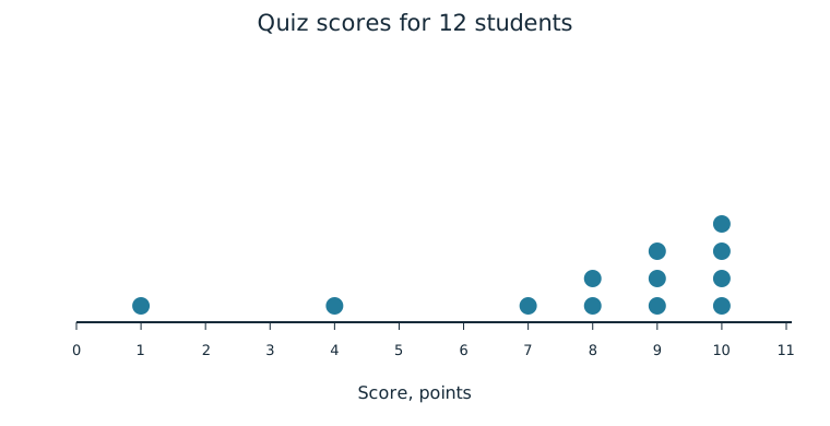
Service times are right/positively skewed because the tail extends farther toward large times. Quiz scores are left/negatively skewed because most scores are high and the tail extends toward small scores. The tallest side alone does not define skew.
| Evidence for credit | Points |
|---|---|
| Both directions with correct larger/smaller-tail reasoning. | 1 |
Peaks and flatness: worked answer
| Bin midpoint | Plot U frequency | Plot B frequency | Plot F frequency |
|---|---|---|---|
| 1 | 1 | 4 | 3 |
| 2 | 3 | 1 | 3 |
| 3 | 6 | 1 | 3 |
| 4 | 3 | 1 | 3 |
| 5 | 1 | 4 | 3 |
Part a
Describe which histogram is unimodal, bimodal, or uniform. Explain the frequency pattern in each.
U has one main peak at midpoint 3 and is unimodal. B has two prominent peaks at 1 and 5 and is bimodal. F has equal frequency 3 in each interval with no prominent peak and is uniform.
| Evidence for credit | Points |
|---|---|
| All three patterns identified and supported. | 1 |
Refute a universal claim: worked answer
Part a
Justify or reject “every sampled customer was served in at most 10 minutes.” Identify graphical evidence and a limit on future claims.
Reject it: dots at 12 and 16 minutes exceed 10. This describes sampled customers; even if no dot exceeded 10, that alone would not guarantee all future customers are served within 10 minutes.
| Evidence for credit | Points |
|---|---|
| Actual plotted counterexamples. | 1 |
| Correct sample versus future scope. | 1 |
Tell the story of tour waits: worked answer
Part a
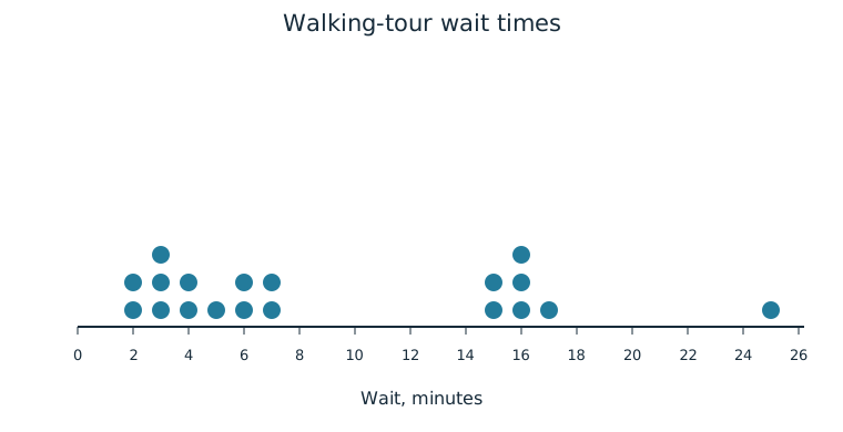
Describe the distribution’s shape, approximate center, and observed variability in context. Include its prominent peaks.
The observed tour waits are right-skewed overall, with prominent peaks around 3 and 16 minutes and clusters at roughly 2–7 and 15–17 minutes. A central observed wait is about 6 minutes, and values range from 2 to 25 minutes. Both clusters matter; a single typical value does not describe the entire pattern.
| Evidence for credit | Points |
|---|---|
| Context and units for center/spread. | 1 |
| Longer right tail, two peaks/clusters, and complete range. | 1 |
Part b
Identify the clusters, at least one gap, and a possible outlier. Explain what each term means using this plot.
Clusters are concentrations near 2–7 and 15–17 minutes. No observations occur between 7 and 15, so that interval is a gap (there is also a gap between 17 and 25). The 25-minute wait is isolated above the rest and a possible outlier; a named numerical rule would be needed for a formal rule-based classification.
| Evidence for credit | Points |
|---|---|
| Clusters as concentrations and gap as empty interval. | 1 |
| Isolated extreme value with appropriately qualified outlier claim. | 1 |
Part c
Justify or reject “all visitors waited less than 20 minutes” and “most sampled waits were below 10 minutes.” Give counts from the graph.
The first is false because one visitor waited 25 minutes. The second is true: 12 of 19 waits are below 10 minutes, more than half. These are statements about the nineteen observed visitors.
| Evidence for credit | Points |
|---|---|
| Counterexample 25 and correct 12/19 majority. | 1 |
| Contextual sampled-visitor scope. | 1 |
Part d
Explain why describing this as an approximately uniform distribution would be misleading.
The counts are concentrated near two separated ranges, with empty intervals and peaks. Frequencies are not approximately equal across ordered values/intervals, so uniformity would hide the clusters and gaps.
| Evidence for credit | Points |
|---|---|
| Uniform condition contrasted with concrete unequal concentrations/gaps. | 1 |