Compare Quantitative Distributions and Relative Position — Worked Solutions
Worked Solutions
Compare your reasoning with the worked solutions after attempting the questions. A different valid representation or explanation can earn credit when it satisfies the stated criteria.
Original generated practice for the Fall 2026 course. Return to the lesson and independent checks.
Compare both samples: worked answer
Part a
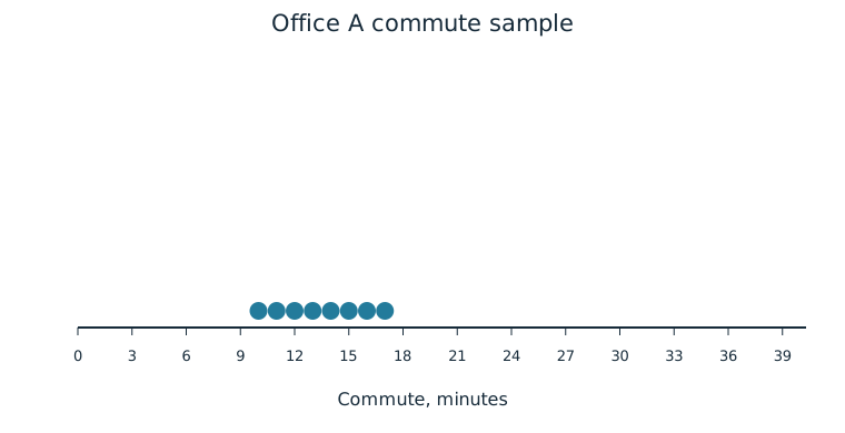
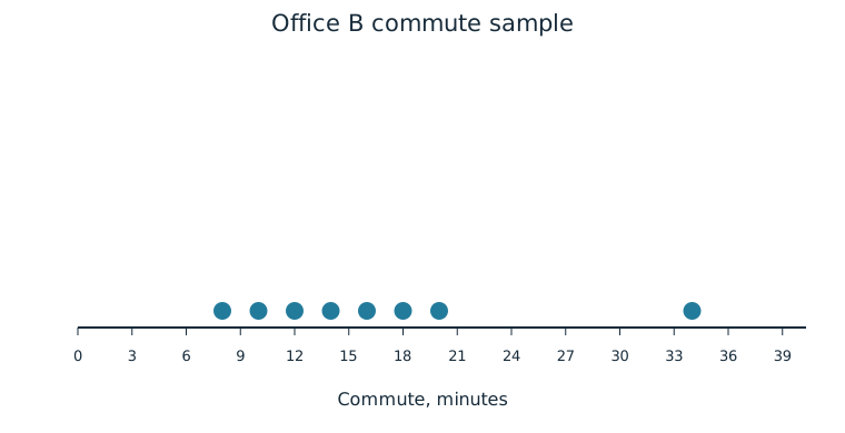
Compare approximate center, spread, shape, clusters/gaps, and unusual values. Include both offices and units.
A is balanced around about 13.5 minutes and spans 10–17. B’s center is somewhat higher (median 15), with much broader 8–34-minute spread and a right tail. B’s main values lie 8–20, with a gap to the isolated 34; A has no comparable internal gap or isolated extreme.
| Evidence for credit | Points |
|---|---|
| Both samples and units for center/spread. | 1 |
| Shape, concentration/gap, and unusual-value contrasts grounded in dots. | 1 |
Add numerical evidence: worked answer
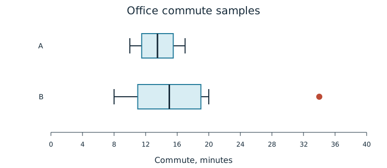
Additional sample summaries: A mean 13.5, SD 2.449; B mean 16.5, SD 8.124. Units are minutes.
Part a
Compare centers and spreads using median, mean, IQR, and SD. Explain the boxplot’s limitation for modes/gaps.
B median 15 exceeds A 13.5 by 1.5 minutes; mean 16.5 exceeds 13.5 by 3. B IQR=8 exceeds A 4, and SD 8.124 exceeds 2.449. Boxplots show positions and outliers but do not identify all internal modes or gaps.
| Evidence for credit | Points |
|---|---|
| All four numerical comparisons with units. | 1 |
| Correct representation limitation. | 1 |
Signed distance: worked answer
A population of test scores has mean 70 points and SD 8 points.
Part a
Calculate and interpret scores 86,62,70 in population-SD units. Define each variable in your formula.
z=(x_i−μ)/σ with data score x_i, population mean μ=70, and population SD σ=8. Scores yield z=2,−1,0: two SDs above, one below, and at the mean. Points cancel in the ratio.
| Evidence for credit | Points |
|---|---|
| Correct formula definitions and three results. | 1 |
| Signs, SD-distance interpretation, and unit cancellation. | 1 |
Absolute and relative can differ: worked answer
Population A has mean 50 and SD 5 points; B mean 80 and SD 20. Individuals score 60 in A and 100 in B.
Part a
Compare absolute scores and relative positions. State why the larger raw score need not have the larger z-score.
100 exceeds 60 absolutely. But A’s score has z=(60−50)/5=2 and B’s has z=(100−80)/20=1, so A stands farther above its own mean in SD units. The reference mean/spread differs.
| Evidence for credit | Points |
|---|---|
| Correct two standardizations. | 1 |
| Both raw and relative comparisons with reference explanation. | 1 |
Build a supported comparison: worked answer
![Counts 6,2,0,0 for bins [0,10),[10,20),[20,30),[30,40).](/statistics-reviewed/data-design/commute-c-independent-hist-v1.svg)
![Counts 4,3,0,1 for bins [0,10),[10,20),[20,30),[30,40).](/statistics-reviewed/data-design/commute-d-independent-hist-v1.svg)
Samples are independent. For population-reference parts only, complete records separately establish μC=8, σC=2 and μD=12, σD=5 minutes. Those population parameters need not equal the sample summaries.
Part a
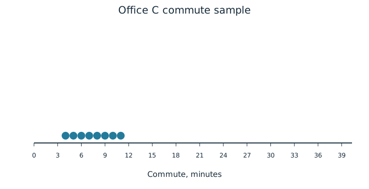
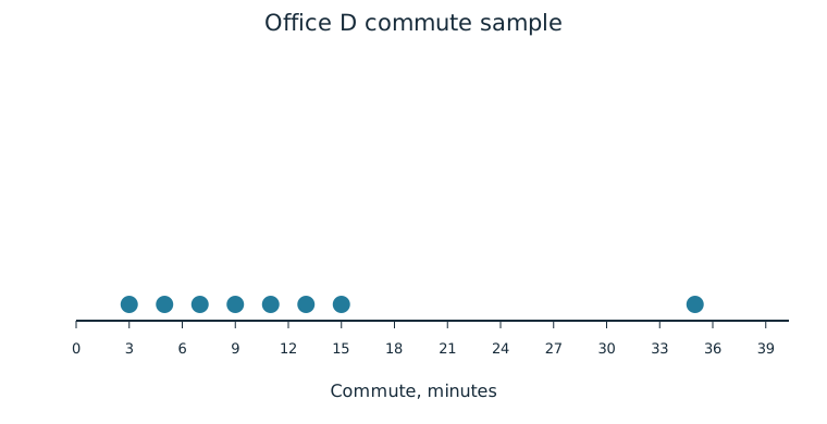
Compare the two distributions using the dots and histograms. Address center, variability, shape, outliers, clusters, and gaps; explain one detail the broad bins hide.
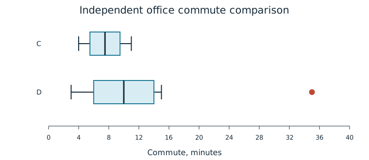
C is relatively balanced around 7.5 minutes, spans 4–11, and has no isolated extreme. D has median 10, spans 3–35, and is right-tailed with a main group 3–15, a long empty gap after 15, and an isolated 35-minute value. Broad 10-minute bins merge distinct individual positions, so the dots reveal the exact gap and within-bin values more clearly.
| Evidence for credit | Points |
|---|---|
| Both samples/units and all required feature comparisons. | 1 |
| Specific grouping limitation rather than false precision from histogram. | 1 |
Part b
Construct a back-to-back stem-and-leaf comparison with tens stems and use it to check the graph comparison. Supply both keys and retain all observations.
C left leaves: stem 0 has 9 8 7 6 5 4; stem 1 has 1 0. D right leaves: 0|3 5 7 9, 1|1 3 5, 2 has none, 3|5. Left stem 1/leaf 1 means 11; right 1|3 means 13 minutes. It confirms C’s compact set and D’s larger range and isolated 35.
| Evidence for credit | Points |
|---|---|
| Complete two-sided exact values and keys. | 1 |
| Comparison supported by constructed representation. | 1 |
Part c
Use the boxplots and calculate mean, median, IQR, and SD to compare samples. Explain why the mean difference is larger than the median difference.
C mean/median=7.5, IQR=4, s=√6≈2.449. D mean=12.25, median=10, IQR=8, s=√100.5≈10.025 minutes. Mean difference is 4.75 minutes, median difference 2.5. D’s high tail/outlier pulls its nonresistant mean more strongly than its median.
| Evidence for credit | Points |
|---|---|
| All summaries and contextual differences. | 1 |
| Tail sensitivity explains mean/median contrast. | 1 |
Part d
Justify or reject “every D commute is longer than every C commute” and “D is more variable.” Name the numerical/graphical evidence and its sample scope.
First claim is false: D includes 3 minutes, below all C observations. Second is supported by IQR 8 vs 4, SD≈10.025 vs 2.449, and range 32 vs 7 minutes. These describe the observed office samples and do not prove the cause of their difference.
| Evidence for credit | Points |
|---|---|
| Concrete counterexample and multiple spread comparisons. | 1 |
| Correct sample/context scope and causal restraint. | 1 |
Part e
Using the known population references, calculate z for C commutes 12,4,8 and D commute 17. Define the variables and interpret every sign.
Use (x_i−μ)/σ. C12 gives 2 (two SD above), C4 gives −2 (two below), C8 gives 0 (at mean). D17 gives 1 (one above). x_i is individual minutes, μ the appropriate population mean, σ its population SD; minutes cancel.
| Evidence for credit | Points |
|---|---|
| Four correct reference-specific calculations. | 1 |
| Definitions, signs, distance, and unit-free interpretation. | 1 |
Part f
Compare C12 with C10 within C, then C12 with D17 between populations. Explain whether the scores alone establish percentile ranks.
C12 has z=2 and C10 z=1, so C12 is farther above C’s mean. D17 has z=1, so despite its larger raw time it is less high relative to its mean/SD than C12. Z-scores alone do not give percentile ranks without distribution-shape information.
| Evidence for credit | Points |
|---|---|
| Within-population and between-population relative comparisons. | 1 |
| Correct raw/relative distinction and percentile limitation. | 1 |
Part g
If C’s population parameters were unknown, standardize its sampled 11-minute observation using sample mean 7.5 and sample SD √6. Explain the fallback and its limit.
Sample-based z=(11−7.5)/√6≈1.429, about 1.429 sample SDs above the sample mean. Sample summaries may be used when population parameters are unknown, but this is not a calculation using known full-population μ/σ and is not automatically a percentile.
| Evidence for credit | Points |
|---|---|
| Correct fallback formula/result and contextual SD distance. | 1 |
| Unknown-parameter and sample-reference distinction. | 1 |