Residuals: Signed Differences and Model Form — Worked Solutions
Worked Solutions
Compare your reasoning with the worked solutions after attempting the questions. A different valid representation or explanation can earn credit when it satisfies the stated criteria.
Original generated practice for the Fall 2026 course. Return to the lesson and independent checks.
Keep the subtraction order: worked answer
A model predicts a 24-minute trip. The observed trip takes 29 minutes.
Part a
Calculate the residual and interpret its sign and size in context. State whether the model underpredicts or overpredicts this trip.
Residual=29−24=5 minutes. The observed trip is 5 minutes longer than predicted, so the model underpredicts this trip’s duration by 5 minutes.
| Evidence for credit | Points |
|---|---|
| Uses observed minus predicted to obtain +5 minutes. | 1 |
| Interprets positive residual as underprediction of trip duration. | 1 |
The model misses high: worked answer
A second trip is predicted to take 24 minutes but actually takes 20 minutes.
Part a
Calculate the residual and explain the model’s error using both the signed residual and the words underpredict or overpredict.
Residual=20−24=−4 minutes. The observation is 4 minutes below the prediction, so the model overpredicts, or overestimates, duration by 4 minutes.
| Evidence for credit | Points |
|---|---|
| Calculates −4 minutes with correct subtraction. | 1 |
| Interprets a negative residual as overprediction with the correct magnitude. | 1 |
Two valid horizontal variables: worked answer
A 3-kilometer route has predicted duration 11 minutes and residual −2 minutes.
Part a
Give its plotted ordered pair when a residual plot uses distance horizontally. Give its ordered pair when predicted duration is horizontal. Identify the vertical variable and its units in both plots.
Against distance, the pair is (3,−2), with x in kilometers. Against predicted duration, the pair is (11,−2), with horizontal minutes. In both cases the vertical variable is residual in minutes; it is neither observed duration nor predicted duration.
| Evidence for credit | Points |
|---|---|
| Gives both correct pairs. | 1 |
| Identifies residual as vertical variable with response units. | 1 |
| Distinguishes the explanatory-value and predicted-response alternatives. | 1 |
Use residual form to assess a line: worked answer
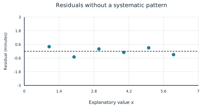
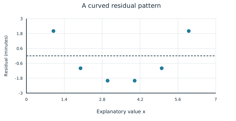
The complete illustrative residual pairs for plots A and B are given in their descriptions. Plot A: (1,0.4),(2,−0.5),(3,0.2),(4,−0.1),(5,0.3),(6,−0.3). Plot B: (1,2),(2,−1),(3,−2),(4,−2),(5,−1),(6,2). Both are residuals from proposed simple linear models.
Part a
Describe each residual pattern and explain what it suggests about linear form. State which better supports a linear model and why the other suggests a different form.
A scatters on both sides of zero without a clear systematic curve, supporting linear form for the observed data. B is U-shaped, with positive residuals at the ends and negative in the middle; this systematic curvature suggests a linear model is not the most appropriate form. A better supports a line, though apparent randomness alone does not verify every model assumption or guarantee predictions.
| Evidence for credit | Points |
|---|---|
| Describes A’s lack of systematic shape and B’s curvature. | 1 |
| Connects random-looking residual scatter to support for linear form. | 1 |
| Connects curvature to a model-form concern, without claiming proof of every assumption. | 1 |
A route model with a hidden curve: worked answer
A delivery service proposes the supplied model , using distance x in kilometers to predict duration y in minutes. The full generated observations follow. The model is a stated proposal, not a claim that its line is the least-squares fit.
| Distance x (km) | Observed time y (min) |
|---|---|
| 1 | 10 |
| 2 | 9 |
| 3 | 10 |
| 4 | 12 |
| 5 | 15 |
| 6 | 20 |
Part a
For all six routes, calculate predicted duration and residual. Display a table with x, observed y, predicted y-hat, and y−y-hat.
Predictions for x=1,2,3,4,5,6 are 7,9,11,13,15,17 minutes. Observations are 10,9,10,12,15,20 minutes, so residuals are 3,0,−1,−1,0,3 minutes. Every residual uses the observation and prediction at the same distance.
| Evidence for credit | Points |
|---|---|
| Calculates all six predictions correctly. | 1 |
| Uses matched observed-minus-predicted differences for all six residuals. | 1 |
| Includes variables and minute units in the table. | 1 |
Part b
Interpret the residuals for the 1-kilometer and 3-kilometer routes. Include direction, size, response units, and whether the model underpredicts or overpredicts.
At 1 kilometer, residual +3 means the route took 3 minutes longer than predicted: the model underpredicts duration by 3 minutes. At 3 kilometers, residual −1 means the route took 1 minute less than predicted: the model overpredicts by 1 minute.
| Evidence for credit | Points |
|---|---|
| Interprets +3 as 3-minute underprediction at the correct route. | 1 |
| Interprets −1 as 1-minute overprediction at the correct route. | 1 |
Part c
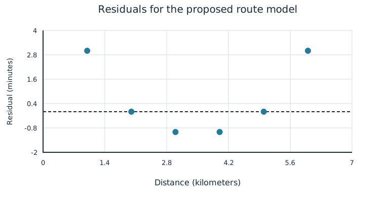
Construct a residual plot against distance. Also list the six ordered pairs you would use if predicted duration were horizontal instead. Label the vertical variable and units.
Against distance plot (1,3),(2,0),(3,−1),(4,−1),(5,0),(6,3). Against predicted duration use (7,3),(9,0),(11,−1),(13,−1),(15,0),(17,3). The vertical variable is residual in minutes in either plot; horizontal units are kilometers in the first and minutes in the second.
| Evidence for credit | Points |
|---|---|
| Constructs all six distance-residual points on labeled axes. | 1 |
| Lists all six correct predicted-duration/residual alternatives. | 1 |
| Uses residual minutes on the vertical axis in both cases. | 1 |
Part d
Describe the form visible in your residual plot and use it to evaluate the proposed linear model. Explain the pattern of underprediction and overprediction across distances.
The residuals have a U-shaped curved pattern: positive at distances 1 and 6, negative at 3 and 4, and zero at 2 and 5. The model underpredicts at the ends and overpredicts in the middle. This systematic curvature suggests a simple linear form is not the most appropriate model for these observations.
| Evidence for credit | Points |
|---|---|
| Describes the curved form and its numerical pattern. | 1 |
| Connects signed residual pattern to underprediction/overprediction across x. | 1 |
| Uses the observed systematic curvature to question the appropriateness of a simple linear form for these routes. | 1 |
Assess a printing-time model: worked answer
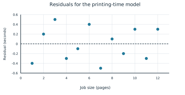
A print shop proposes the supplied linear model , using job size x in pages to predict printing time y in seconds. Twelve complete generated observations and their matched observed-minus-predicted residuals are supplied below. These are a diagnostic check of the stated model; its fixed coefficients are not claimed to be the least-squares fit to this sample.
| Job size x (pages) | Observed time y (seconds) | Predicted time (seconds) | Residual y−predicted (seconds) |
|---|---|---|---|
| 1 | 9.6 | 10 | -0.4 |
| 2 | 12.2 | 12 | 0.2 |
| 3 | 14.5 | 14 | 0.5 |
| 4 | 15.7 | 16 | -0.3 |
| 5 | 17.9 | 18 | -0.1 |
| 6 | 20.4 | 20 | 0.4 |
| 7 | 21.5 | 22 | -0.5 |
| 8 | 24.1 | 24 | 0.1 |
| 9 | 25.8 | 26 | -0.2 |
| 10 | 28.3 | 28 | 0.3 |
| 11 | 29.7 | 30 | -0.3 |
| 12 | 32.3 | 32 | 0.3 |
Part a
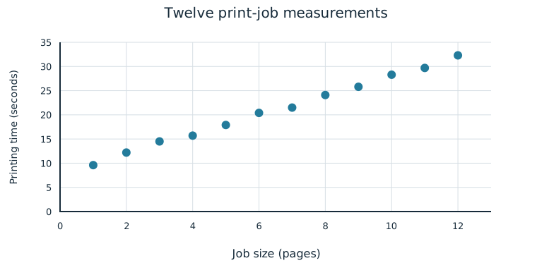
Describe the form of the original printing-time-versus-job-size association. Cite the plotted observations to decide whether a linear trend is present and a straight-line form is reasonable to investigate.
The original measurements show an approximately straight increasing trend: for example, observed time rises from 9.6 seconds at 1 page to 20.4 seconds at 6 pages and 32.3 seconds at 12 pages, with the other jobs close to the same straight path. The data exhibit an approximately linear trend, so a simple linear form is reasonable to investigate rather than fitting one to an obviously curved association. This initial plot does not establish every modeling assumption.
| Evidence for credit | Points |
|---|---|
| Describes an approximately linear increasing trend in job size and printing time. | 1 |
| Uses actual plotted values or the overall straight pattern to justify investigating a linear form. | 1 |
Part b
Describe the residual plot’s form and how the residuals are arranged relative to zero. Use that pattern to evaluate the supplied simple linear model for these observed jobs. Cite specific plotted evidence and state one limitation of what the diagnostic establishes.
The residuals lie on both sides of zero, ranging from −0.5 to +0.5 seconds, without a clear systematic curve or trend across job size. For example, at 3 pages the residual is +0.5 seconds, at 7 pages it is −0.5, and near the upper end the 10/11/12-page residuals are +0.3/−0.3/+0.3 seconds. Their apparent pattern-free scatter, together with the approximately linear original-data trend, supports the linear form as appropriate for these observed jobs. It does not prove that all assumptions hold, guarantee each prediction, or establish a cause-and-effect mechanism. Equivalent descriptions of the apparent lack of a systematic pattern can earn credit.
| Evidence for credit | Points |
|---|---|
| Describes residuals above and below zero without a clear systematic curve or trend, citing correct point/sign evidence from this fresh plot. | 1 |
| Connects apparent randomness and the approximately linear original-data trend to support for the supplied linear form for these observed jobs. | 1 |
| States a valid diagnostic limitation without contradicting the supported linear-form conclusion. | 1 |