1.1 Categorical Data
Section Overview
- Gallery 1.1.1 - Joint and Marginal Dist.
- Gallery 1.1.2 - Cond. Frequencies and Dist.
- Example 1.1.1
- Pop Quiz 1.1.1
Quantitative vs Categorical Variables
We will discuss two types of variables that you will encounter in Statistics and everyday life in general. There are quantitative variables, which have numerical values that measure some characteristic of a person or thing. Some examples could include: the strength of an alligator’s bite measured in Newtons (N), the speed at which you race down a hill in a shopping cart measured in kilometers per hour (km/h), or the degree of frustration you feel for Statistics measured in number of times you bang your head onto your desk (hopefully that will change by the end of this guide!)
In this section, however, we’ll be focusing on qualitative variables, which are also commonly called categorical variables. As the name suggests, the values for categorical variables are categories instead of numbers. Some examples could include: your friend’s favorite type of pizza toppings “measured” in sardines, pineapples, and peanut butter and your favorite subjects in school “measured” in physics, history, chemistry, and statistics.
Distributions of Categorical Variables
You’ve probably heard of pie charts and bar graphs, right? These are the most common ways to display the distribution of categorical data, where the distribution describes what values the variable can take and how frequently the variable takes them. Speaking of “frequent”, we can also display the distribution of a categorical variable in a frequency table, which records the number in each category. Alternatively, you can use a relative frequency table, which records the percent in each category.
To put our newfound knowledge to use, let’s assume that the Sales Manager of a local candy company wanted to find out how many boxes have been sold for each of their nine flavors of candy since last week. The results can be seen in the following frequency and relative frequency tables:
Frequency Table
| Candy Flavor | Count |
|---|---|
| Bombastic Blueberry | 4826 |
| Caramel Crush | 5362 |
| Gravitational Grape | 3537 |
| Lickety Lime | 4081 |
| Mouthwatering Marshmallow | 3925 |
| Omnom Orange | 5911 |
| Pleasant Peach | 2678 |
| Rowdy Raspberry | 3384 |
| Wicked Watermelon | 4690 |
| Total | 38394 |
Relative Frequency Table
| Candy Flavor | Percent |
|---|---|
| Bombastic Blueberry | 12.6% |
| Caramel Crush | 14.0% |
| Gravitational Grape | 9.2% |
| Lickety Lime | 10.6% |
| Mouthwatering Marshmallow | 10.2% |
| Omnom Orange | 15.4% |
| Pleasant Peach | 7.0% |
| Rowdy Raspberry | 8.8% |
| Wicked Watermelon | 12.2% |
| Total | 100% |
The distribution of values for each flavor can also be seen in the following pie chart and bar graph:
Marginal and Joint Frequencies
We’ve just learned a couple of tricks for displaying the distribution for a single categorical variable. What do we do when two categorical variables are involved? We create something called a two-way table, which, like the frequency tables, can display counts or percents. It might be a bit difficult to visualize, so let’s start with another example: A survey that was randomly given to a very small number of select players on a large MMORPG (Massively Multiplayer Online Role Playing Game) server asked them to indicate their gender and the class of their character (Knight, Ninja, Archer, Wizard, and Healer). The results are shown in the following two-way tables:
| Class | Male | Female | Total |
|---|---|---|---|
| Knight | 752 | 403 | 1155 |
| Ninja | 611 | 445 | 1056 |
| Archer | 386 | 254 | 640 |
| Wizard | 460 | 655 | 1115 |
| Healer | 141 | 369 | 510 |
| Total | 2350 | 2126 | 4476 |
| Class | Male | Female | Total |
|---|---|---|---|
| Knight | 16.8% | 9.0% | 25.8% |
| Ninja | 13.7% | 9.9% | 23.6% |
| Archer | 8.6% | 5.7% | 14.3% |
| Wizard | 10.3% | 14.6% | 24.9% |
| Healer | 3.2% | 8.2% | 11.4% |
| Total | 52.5% | 47.5% | 100% |
Similar to when we were examining single categorical variables, parts of a two-way table can be translated into graphs. The green and light green entries in the body of the table are joint frequencies, which record the counts of individuals that jointly fall into both categories. The joint relative frequencies in the second table record the count of these individuals out of the overall total, or:
All of the other colored entries in the margins of the table that record total counts are called — you guessed it — marginal frequencies. There are two sets of marginal frequencies. There is the set that counts the total number of players in each class. There is also the set that counts the total number of players for each gender, represented by the blue and purple entries. Again, marginal relative frequencies record the totals out of the overall total, or:
As promised, the joint distribution and both sets of marginal distributions can also be seen in the following graphs:
Gallery 1.1.1 Joint and Marginal Distribution
Frame 1 of 3
The joint distribution of the MMORPG problem. Open full-size image S0007Frame 2 of 3
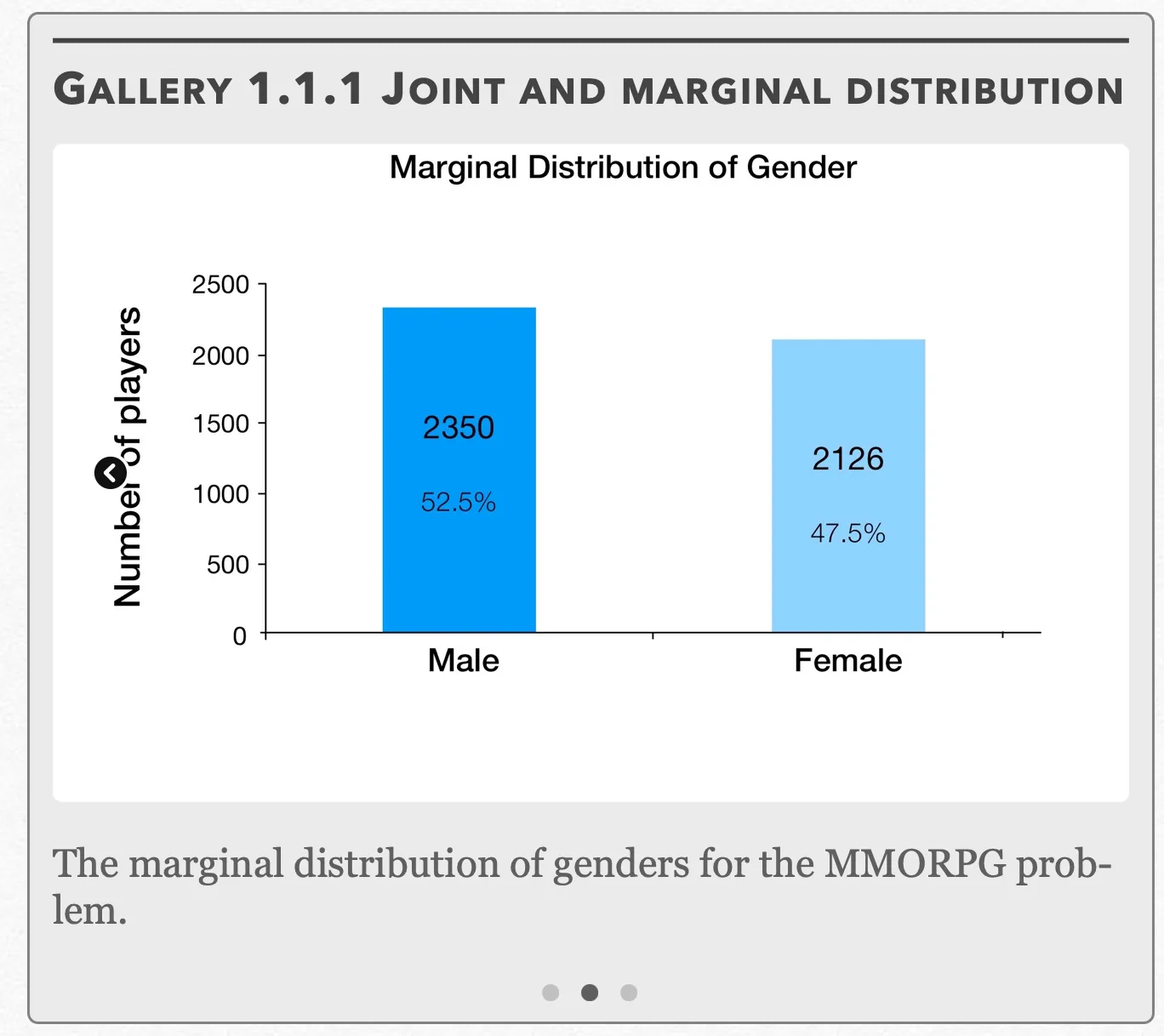
The marginal distribution of genders for the MMORPG problem. Open full-size image S0009Frame 3 of 3
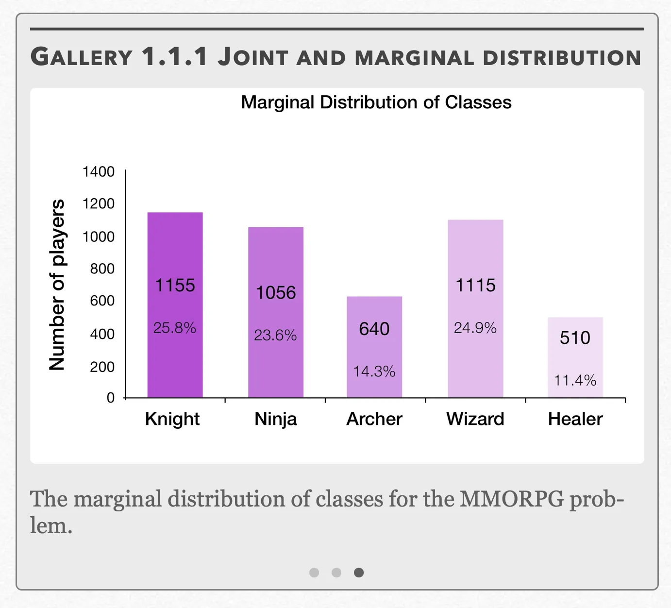
The marginal distribution of classes for the MMORPG problem. Open full-size image S0008
Capture provenance
Filename capture times, with no recorded timezone. Frames above follow the original gallery positions.
- · S0007 · displayed frame 1
Screenshot 2026-10-05 at 3.36.32 PM.png - · S0008 · displayed frame 3
Screenshot 2026-10-05 at 3.37.02 PM.png - · S0009 · displayed frame 2
Screenshot 2026-10-05 at 3.37.10 PM.png
Conditional Relative Frequencies
Maybe it seems like we’ve already beaten the concept of frequencies to death in this section. But we’re not done yet. We still have conditional relative frequencies to cover, which record the count of individuals out of the totals from one of the categories. In other words:
As there are two different distributions of marginal frequencies, there are two sets of conditional relative frequencies that could be represented in each of the cells. This problem can be solved by creating two sets of conditional relative frequency tables, which each also getting their own conditional distribution graphs:
Gallery 1.1.2 Conditional Frequencies and Distributions
Frame 1 of 4
The conditional relative frequencies of classes within each gender. Open full-size image S0010Frame 2 of 4
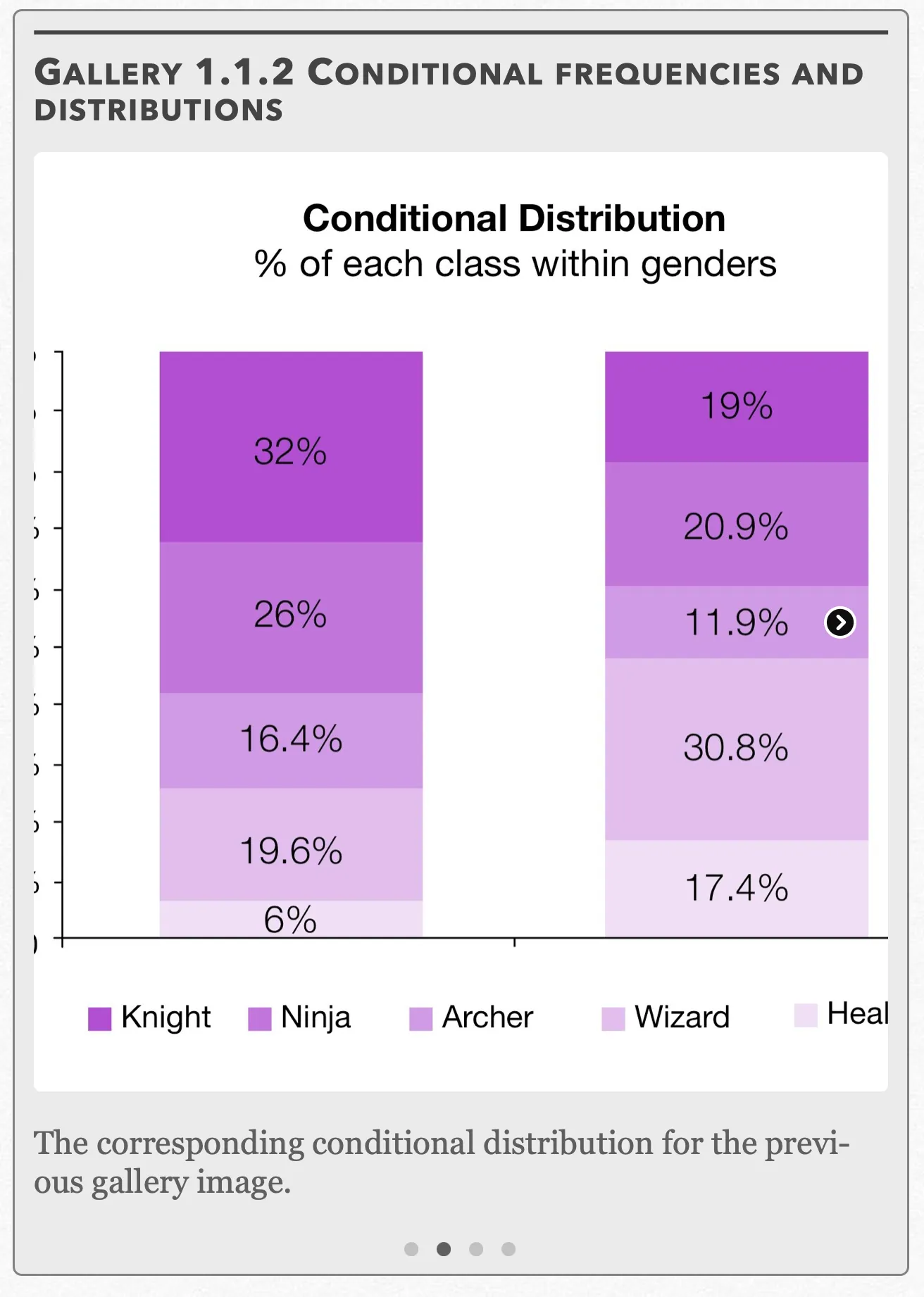
The corresponding conditional distribution for the previous gallery image. Open full-size image S0011Frame 3 of 4
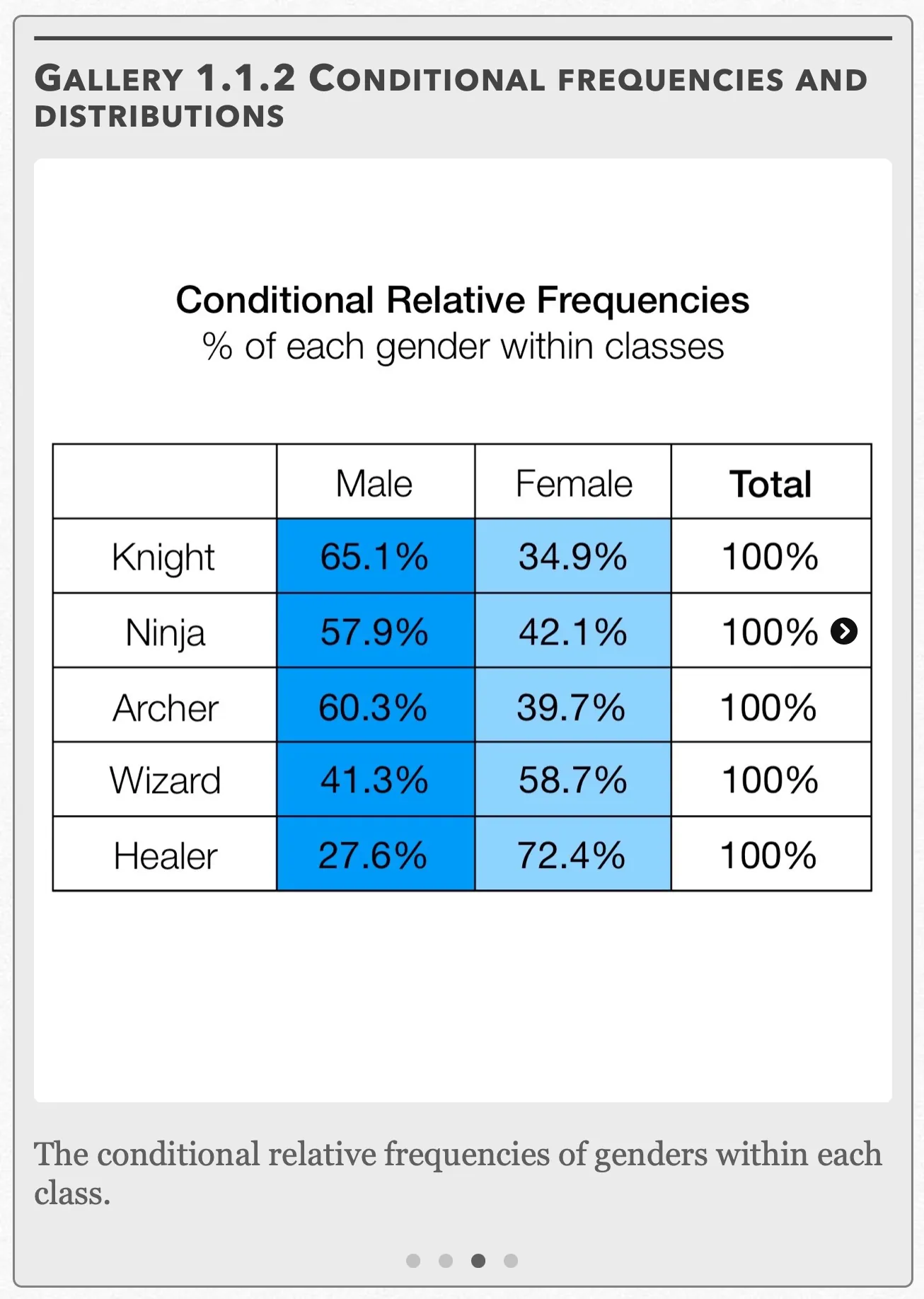
The conditional relative frequencies of genders within each class. Open full-size image S0012Frame 4 of 4
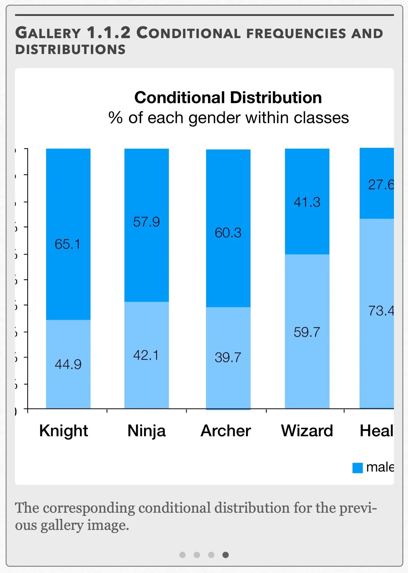
The corresponding conditional distribution for the previous gallery image. Open full-size image S0013
Capture provenance
Filename capture times, with no recorded timezone. Frames above follow the original gallery positions.
- · S0010 · displayed frame 1
Screenshot 2026-10-05 at 3.37.15 PM.png - · S0011 · displayed frame 2
Screenshot 2026-10-05 at 3.37.23 PM.png - · S0012 · displayed frame 3
Screenshot 2026-10-05 at 3.37.29 PM.png - · S0013 · displayed frame 4
Screenshot 2026-10-05 at 3.37.34 PM.png
Conditional Relative Frequencies: % of each class within genders
| Class | Male | Female |
|---|---|---|
| Knight | 32.0% | 19.0% |
| Ninja | 26.0% | 20.9% |
| Archer | 16.4% | 11.9% |
| Wizard | 19.6% | 30.8% |
| Healer | 6.0% | 17.4% |
| Total | 100% | 100% |
Conditional Relative Frequencies: % of each gender within classes
| Class | Male | Female | Total |
|---|---|---|---|
| Knight | 65.1% | 34.9% | 100% |
| Ninja | 57.9% | 42.1% | 100% |
| Archer | 60.3% | 39.7% | 100% |
| Wizard | 41.3% | 58.7% | 100% |
| Healer | 27.6% | 72.4% | 100% |
Let’s review what we’ve learned so far with an example problem:
Example 1.1.1 — recorded solution
a) We want to find the number of players that (1) are female and (2) play the Ninja class. Looking across the “Ninja” row and under the “Female” column, we see there are 445 such players.
We want to find the percentages of these players out of the overall total on the server, so we use:
9.9% of players on the server are female Ninjas.
b) Notice how this question is phrased slightly differently from the one in (a). Instead of the entire population of people on the server, we should only be looking at the “Ninja population”. There are 1056 Ninjas on the server and 445 of those Ninjas are female. Since 445 is a joint frequency and 1056 is a marginal frequency, this lets us know immediately that we should use the conditional relative frequency formula:
42.1% of Ninjas are female.
c) Unlike in (b), the specific population we’re looking at this time is the female population. Out of 2126 female players on the server, 445 are female. Again we use the conditional relative frequency formula:
20.9% of females are Ninjas.
d) There are 1056 Ninjas that play on the server and 4476 overall players on the server. If we’re looking at the entire population instead of one of the smaller “subpopulations”, this means we use:
23.6% percent of people play Ninjas.
e) For the uninitiated, character classes in MMORPG’s each have their own roles to play within the greater scope of the game. Looking at the graphs of both conditional distributions, we can see males tending to favor the more weapons-based classes consisting of Knights, Ninjas, and Archers and females tending to favor the more magic-based classes consisting of Wizards and Healers. This provides evidence for an association, or a relationship between the two variables, gender and character class.
Pop Quiz 1.1.1
Glossary and deeper reading · 13 refreshers
These editorial refreshers supplement the reading. Definitions and examples are added guidance; original source wording and recorded answers remain in their original context.
-
Quantitative variable
A quantitative variable records a numerical count or measurement for each individual. Differences between its values have a meaningful numerical interpretation. For example, the number of books borrowed and the mass of a backpack are quantitative variables.
-
Categorical variable
A categorical variable records a group or label for each individual. Numeric labels still count as categories when arithmetic on them has no meaningful interpretation. For example, favorite school subject is categorical, even if each subject receives a numbered code.
-
Pie chart
A pie chart displays category proportions as slices of a circle. A slice’s angle is proportional to its category’s share of the whole. For example, a category containing one quarter of the observations occupies one quarter of the circle.
-
Bar graph
A bar graph uses separate bars to compare category counts or proportions. The bar lengths or heights encode the values, and category order need not be numerical. For example, separate bars can compare the number of votes for three lunch options.
-
Relative frequency
Relative frequency is a group’s count divided by the total count. It can be written as a proportion or multiplied by 100 to give a percentage. For example, 8 choices out of 20 have relative frequency 0.4, or 40%.
-
Frequency table
A frequency table lists the number of observations in each category or numerical interval. Its counts add to the total number of observations when the groups do not overlap and cover all observations. For example, a table can record how many students chose each lunch option.
-
Survey
A survey collects information by asking individuals questions. Its quality depends on the sample design, question wording, and responses received. For example, a school can survey selected families about their transportation needs.
-
Joint frequency
A joint frequency is the count in one cell of a two-way table. It counts individuals who meet both the row category and the column category. For example, a cell might count students who are in grade 11 and walk to school.
-
Joint relative frequency
A joint relative frequency divides one cell’s count by the overall table total. It describes the proportion of all individuals who have both listed characteristics. For example, 6 grade-11 walkers among 30 students give a joint relative frequency of 20%.
-
Marginal frequency
A marginal frequency is a row or column total in a two-way table. It counts one category without separating individuals by the other variable. For example, the total number of walkers includes walkers from every grade level.
-
Marginal relative frequency
A marginal relative frequency divides a row or column total by the overall table total. The collection of these proportions describes one categorical variable on its own. For example, 12 walkers among 30 students give a marginal relative frequency of 40%.
-
Joint distribution
A joint distribution describes the combinations of values of two variables and how often they occur. For categorical data it can be represented by cell counts or proportions in a two-way table. For example, the distribution of students across grade-level and transportation-mode combinations is a joint distribution.
-
Marginal distribution
A marginal distribution describes one variable on its own after the other variable is summed or otherwise accounted for. In a two-way table, it uses row or column totals, expressed as counts or proportions. For example, adding all grade-level counts for each transportation mode gives the marginal distribution of transportation mode.