1.3 Numerical Summaries of Quantitative Data
Section Overview
- Gallery 1.3.1 - Boxplot Symmetries
- Gallery 1.3.2 - 5 # Sum. & Boxplots on Calc
- Example 1.3.1
- Interactive 1.3.1 - Example 1.3.1
- Pop Quiz 1.3.1
Introduction to Boxplots
Previously, we discussed using numbers to describe aspects of a distribution, such as the range to describe the spread and the median to describe the center. In this section, we’ll be introducing additional ways to describe the shape, center, spread, and any unusual features for a different type of graph: the boxplot (also called a box-and-whisker plot).
Shape — The shape of a boxplot can be described in terms of its symmetry like the other graphs. A boxplot is left-skewed if the observations to the left of (or smaller than) the median are more varied from one another than the observations to the right of (or larger than) the median, and vice versa for right-skewed. Of course, a boxplot is symmetric if the observations are evenly varied on either side of the median. However, we can no longer use peaks to describe shape because a boxplot lacks the capability to display them. Examples of boxplots with differing symmetries can be seen in Gallery 1.3.1.
Center — We can still use the median as a measure of center for a boxplot. We can compare this to another measure of center, the mean, which is also written as . The mean can be calculated as follows:
Spread — Expanding on the range, we have the Interquartile Range (IQR), or the difference between the 1st quartile (Q₁) and the 3rd quartile (Q₃), or
Q₁ is the median of the values that are smaller than the median proper when the observations are numbered from least to greatest. Similarly, Q₃ is the median of the values that are greater than the median proper when the observations are numbered from least to greatest. We also introduce the standard deviation, which is also written as ; it is roughly the average distance of the values of the observations from the mean. The square of the standard deviation is called the variance, or .
Unusual Features — In this section, we can formally call an observation an outlier if:
Gallery 1.3.1 Boxplot Symmetries
Frame 1 of 3
An example of a right-skewed boxplot. Notice how there are NOT more values to the right of the median, but that the values to the right of the median are more varied from one another than values on the left side of the median. Open full-size image S0040Frame 2 of 3
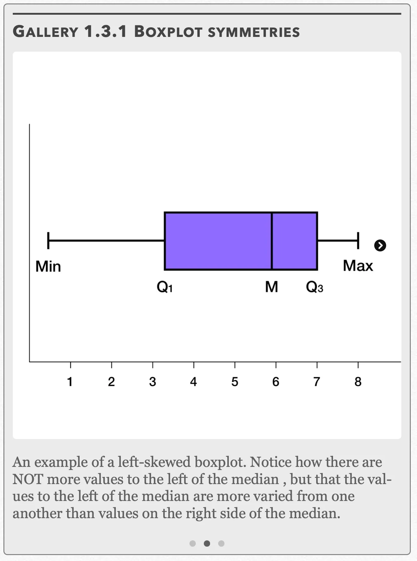
An example of a left-skewed boxplot. Notice how there are NOT more values to the left of the median, but that the values to the left of the median are more varied from one another than values on the right side of the median. Open full-size image S0041Frame 3 of 3
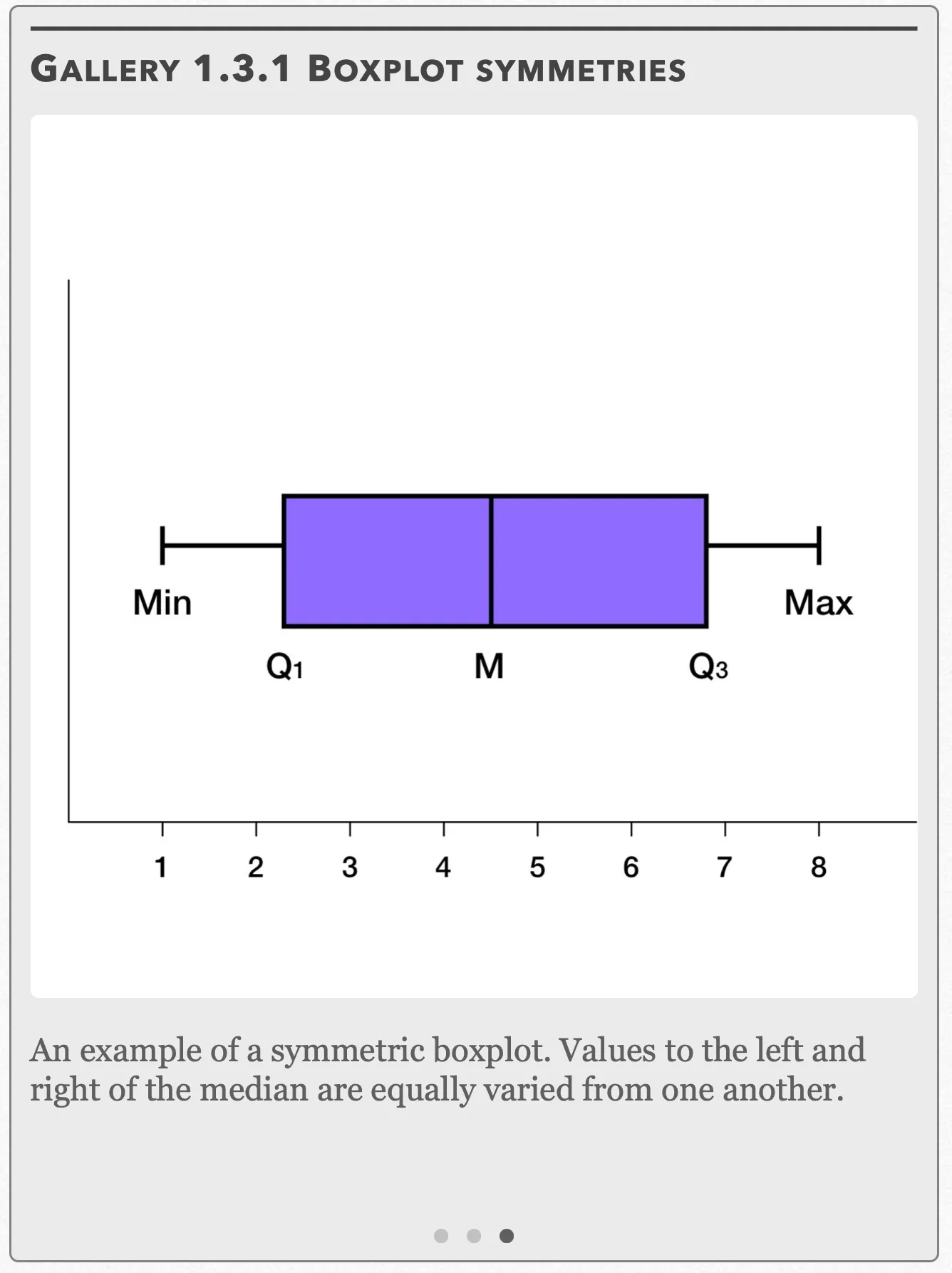
An example of a symmetric boxplot. Values to the left and right of the median are equally varied from one another. Open full-size image S0042
Capture provenance
Filename capture times, with no recorded timezone. Frames above follow the original gallery positions.
- · S0040 · displayed frame 1
Screenshot 2026-10-05 at 3.39.19 PM.png - · S0041 · displayed frame 2
Screenshot 2026-10-05 at 3.39.25 PM.png - · S0042 · displayed frame 3
Screenshot 2026-10-05 at 3.39.31 PM.png
Creating the Boxplot
We can sketch a boxplot if we know the smallest observation (the minimum), the largest observation (the maximum), Q₁, Q₃, and the median of a distribution, also called its five-number summary. The box is made up of the two quartiles and the median, and whiskers are made up of the smallest and largest observations. If the largest or smallest observations also happen to be outliers, then we use a dot to represent the outlier and use the next largest or smallest observations to make up the whiskers. Refer to Gallery 1.3.2 for learning how to create a boxplot on the calculator.
Gallery 1.3.2 Example 1.3.1 (5-Number Summary and Graphing Boxplots on TI-83/84)
Frame 1 of 9
Press the STAT button and under EDIT, select “Edit” and press ENTER Open full-size image S0043Frame 2 of 9
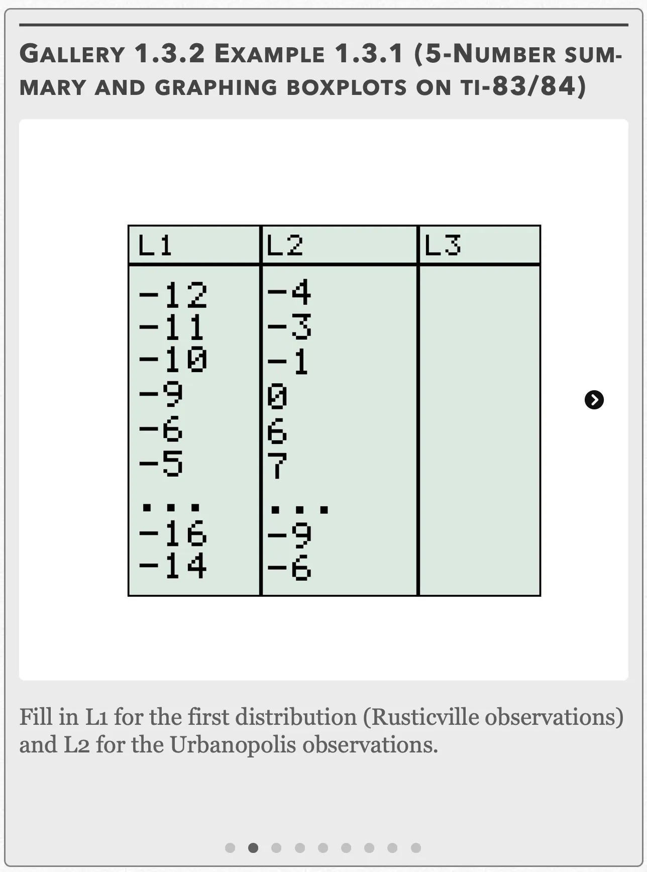
Fill in L1 for the first distribution (Rusticville observations) and L2 for the Urbanopolis observations. Open full-size image S0044Frame 3 of 9
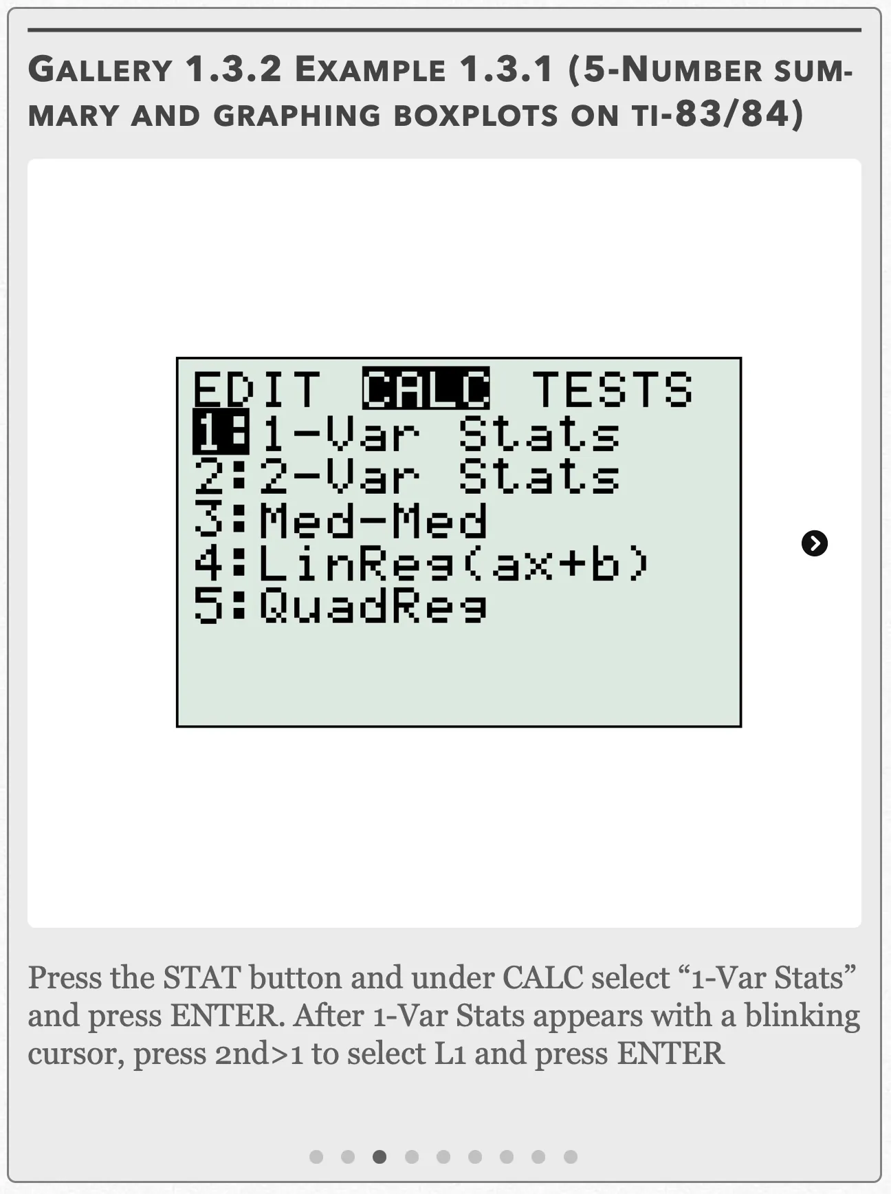
Press the STAT button and under CALC select “1-Var Stats” and press ENTER. After 1-Var Stats appears with a blinking cursor, press 2nd>1 to select L1 and press ENTER Open full-size image S0045Frame 4 of 9
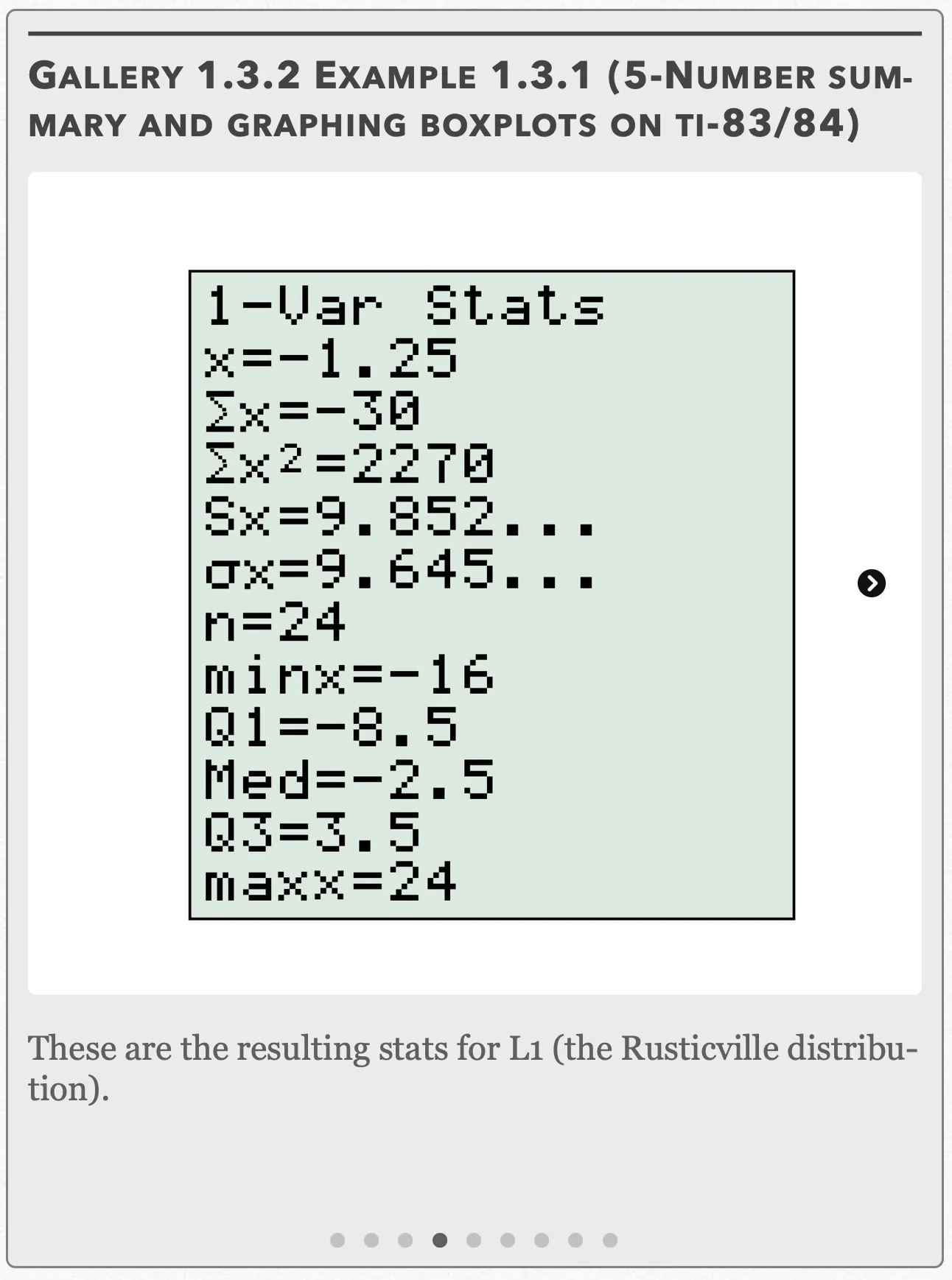
These are the resulting stats for L1 (the Rusticville distribution). Open full-size image S0046Frame 5 of 9
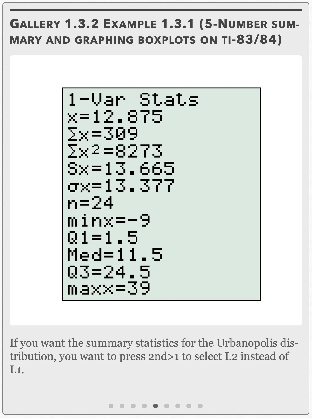
If you want the summary statistics for the Urbanopolis distribution, you want to press 2nd>1 to select L2 instead of L1. Open full-size image S0047Frame 6 of 9
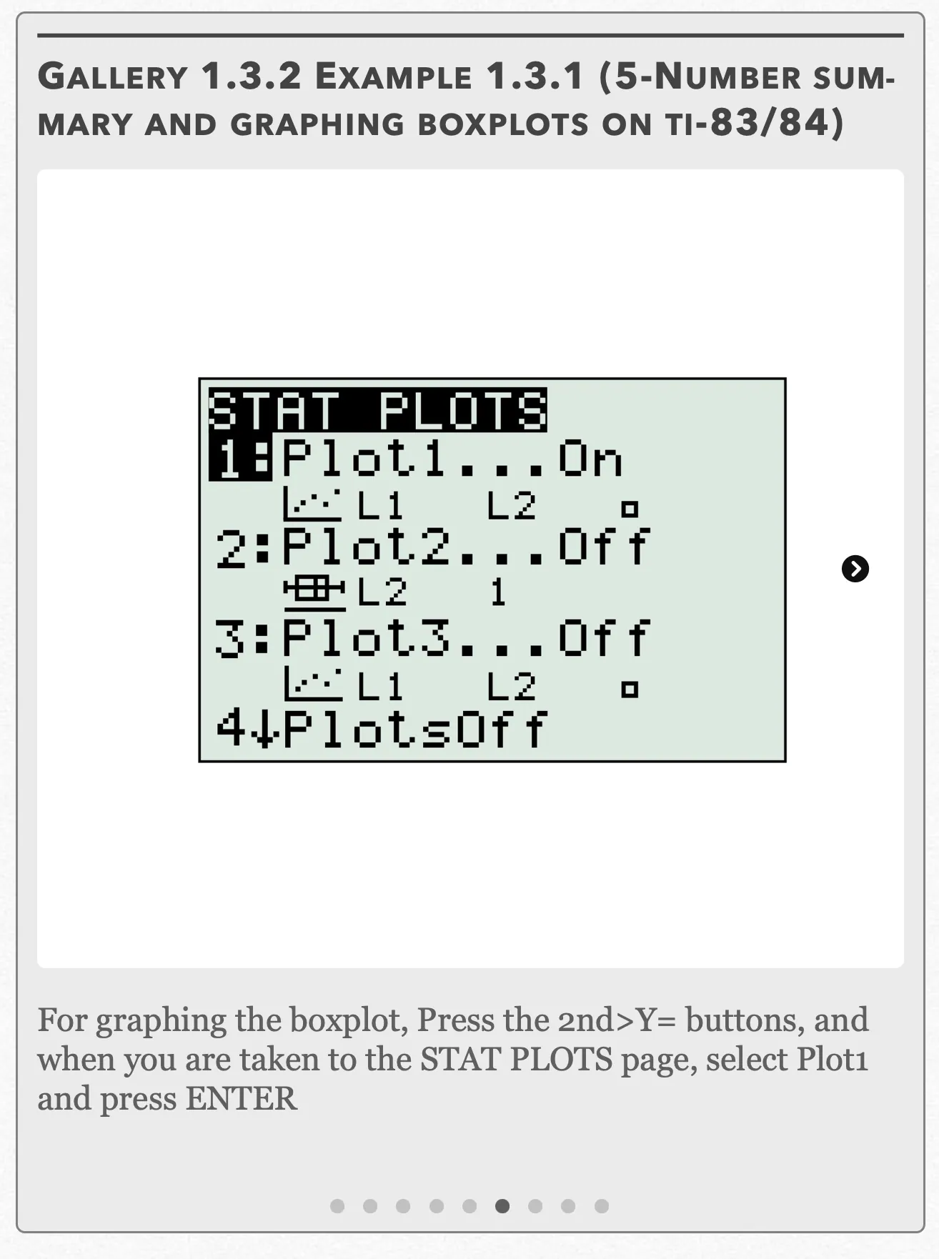
For graphing the boxplot, Press the 2nd>Y= buttons, and when you are taken to the STAT PLOTS page, select Plot1 and press ENTER Open full-size image S0048Frame 7 of 9
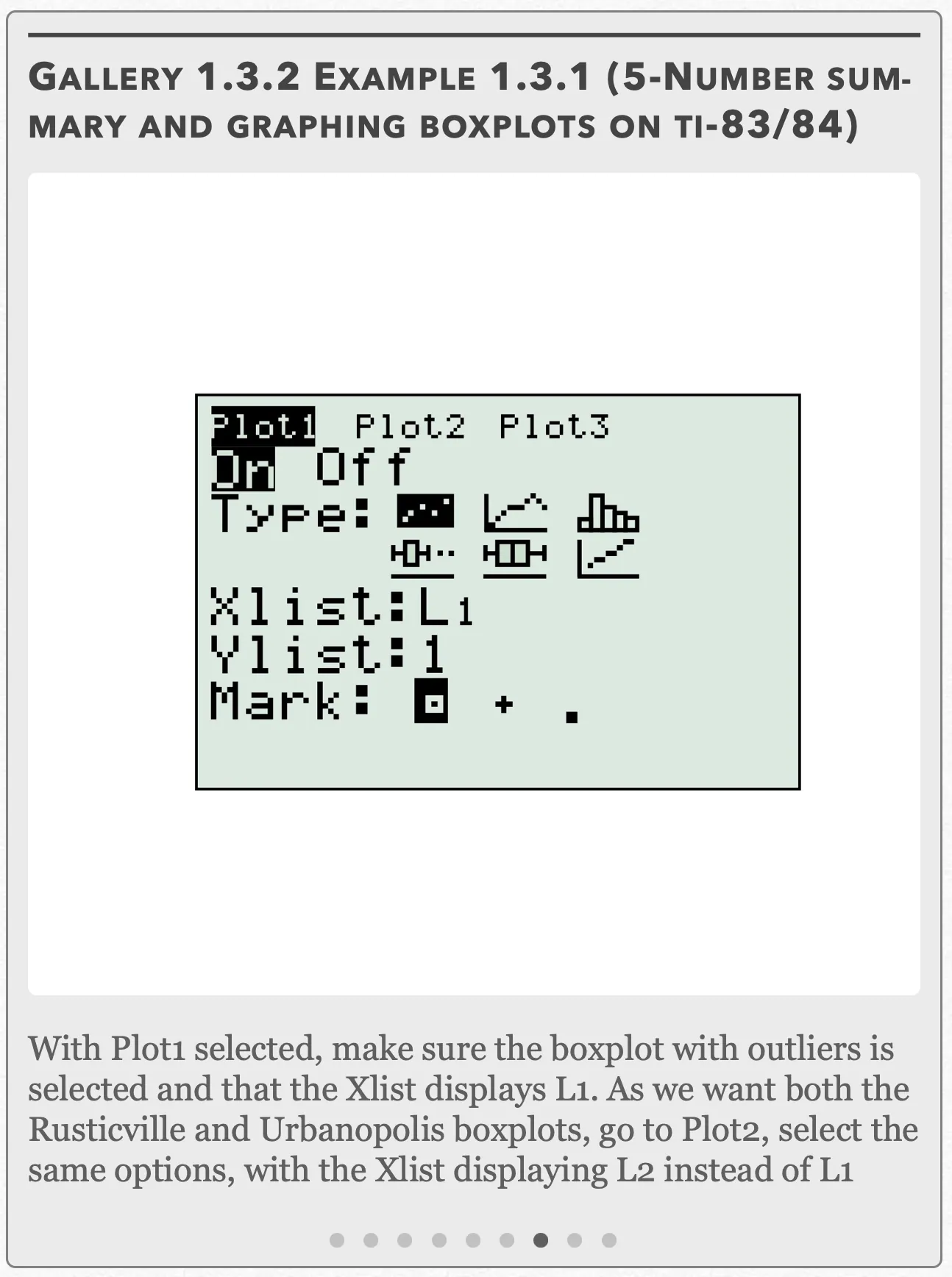
With Plot1 selected, make sure the boxplot with outliers is selected and that the Xlist displays L1. As we want both the Rusticville and Urbanopolis boxplots, go to Plot2, select the same options, with the Xlist displaying L2 instead of L1 Open full-size image S0049Frame 8 of 9
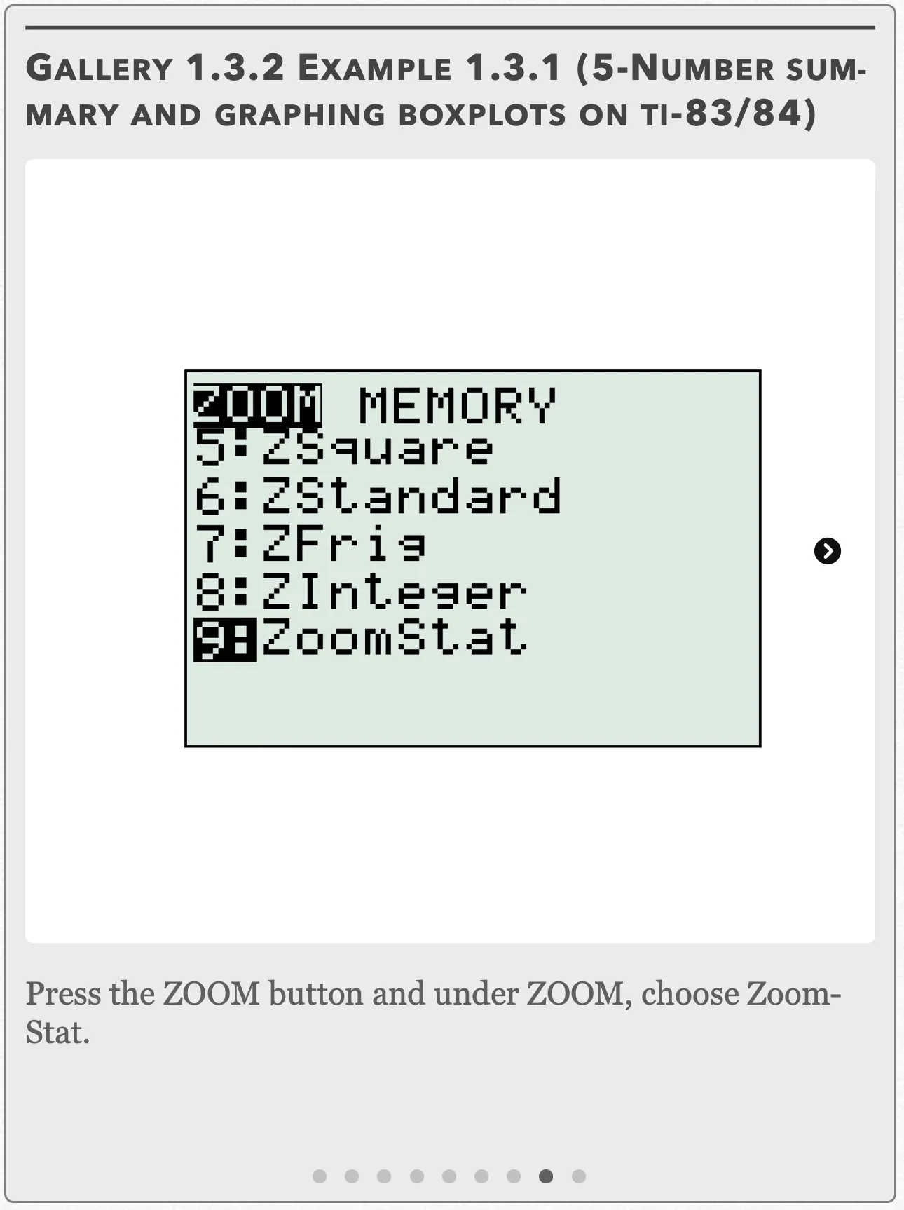
Press the ZOOM button and under ZOOM, choose ZoomStat. Open full-size image S0050Frame 9 of 9
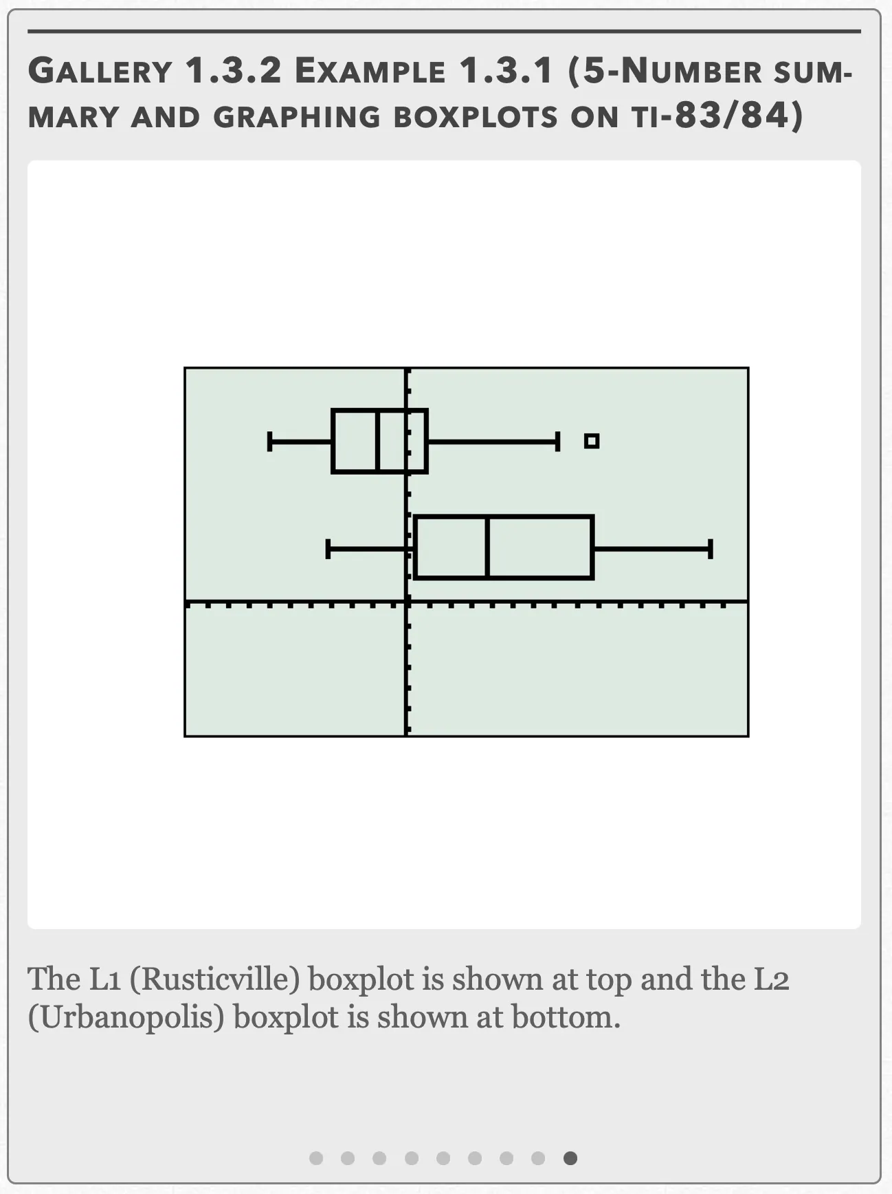
The L1 (Rusticville) boxplot is shown at top and the L2 (Urbanopolis) boxplot is shown at bottom. Open full-size image S0051
Capture provenance
Filename capture times, with no recorded timezone. Frames above follow the original gallery positions.
- · S0043 · displayed frame 1
Screenshot 2026-10-05 at 3.39.38 PM.png - · S0044 · displayed frame 2
Screenshot 2026-10-05 at 3.39.44 PM.png - · S0045 · displayed frame 3
Screenshot 2026-10-05 at 3.39.48 PM.png - · S0046 · displayed frame 4
Screenshot 2026-10-05 at 3.39.53 PM.png - · S0047 · displayed frame 5
Screenshot 2026-10-05 at 3.39.59 PM.png - · S0048 · displayed frame 6
Screenshot 2026-10-05 at 3.40.04 PM.png - · S0049 · displayed frame 7
Screenshot 2026-10-05 at 3.40.09 PM.png - · S0050 · displayed frame 8
Screenshot 2026-10-05 at 3.40.15 PM.png - · S0051 · displayed frame 9
Screenshot 2026-10-05 at 3.40.21 PM.png
Recorded calculator statistics
| Statistic | L1: Rusticville | L2: Urbanopolis |
|---|---|---|
| Mean, x̄ | −1.25 | 12.875 |
| Σx | −30 | 309 |
| Σx² | 2270 | 8273 |
| Sx | 9.852… | 13.665 |
| σx | 9.645… | 13.377 |
| n | 24 | 24 |
| minX | −16 | −9 |
| Q1 | −8.5 | 1.5 |
| Med | −2.5 | 11.5 |
| Q3 | 3.5 | 24.5 |
| maxX | 24 | 39 |
Resistant Measures
When we look at a boxplot and determine its symmetry, we can also determine what measures of center and spread are best for describing the distribution. If the boxplot is skewed and/or has outliers, then we should use the median and the IQR. This is because the median and the IQR are resistant measures of center and spread, or unaffected by extreme observations.
To illustrate this: if you list the observations in a distribution from least to greatest and change the value of every observation except for the median or either of the two quartiles, the values of the median and the IQR do not budge (assuming the values you changed don’t force you to reorder the distribution and declare a new median!) This also applies to Q₁ and Q₃, the two measures that make up the IQR, since they are also medians within the distribution.
Otherwise, use the mean and the standard deviation to describe the distribution. This is especially important when comparing parallel boxplots, or two boxplots shown side-by-side.
Example 1.3.1 — recorded solution
a) Shape: When the boxplot is sketched by hand or generated on a calculator (refer to Gallery 1.3.2), we can see that the Rusticville and Urbanopolis distributions are both right-skewed.
b) Center: The distributions are skewed, so we will use the median as our measure of center. There is an even number of observations for both distributions, so the median will be the average of the two innermost observations. When the observations are ordered from least to greatest, we find the median for the Rusticville observations to be −2.5°C and 11.5°C for the Urbanopolis observations.
We can also use the calculator to find these values (See Gallery 1.3.2). On the same screen, you should find the means for each distribution, calculated to be for Rusticville and for Urbanopolis.
c) Spread: The distributions are skewed, so we will use the IQR as our measure of spread.
For Rusticville, and , making our
For Urbanopolis, and , making our .
We can also use the calculator to find these values as shown in Gallery 1.3.2. On the same screen, you should find the standard deviations for each distribution, calculated to be for Rusticville and for Urbanopolis.
d) Unusual Features: We can find any outliers by plugging Q₁, Q₃, the IQR, and the largest and smallest observations into the outlier inequality:
If the inequality is true, then the observation is an outlier. For Rusticville we have:
Only the second inequality is true, so 23°C is the outlier for the Rusticville distribution.
For Urbanopolis, we have:
Neither of the inequalities are true, so there are no outliers for the Urbanopolis distribution.
Looking at the two boxplots, we see that Rusticville in general has much cooler weather than Urbanopolis, but we also see that the weather also varies less in Rusticville than in Urbanopolis. When making the decision of which city to move to, you have to take these factors into consideration. For instance, if you liked warm weather, but due to your crippling college debt could only afford a tiny studio apartment, then you might want to move to Rusticville, since you’d probably likely only be wearing warm clothing there.
Interactive 1.3.1 Example 1.3.1
Pop Quiz 1.3.1
Glossary and deeper reading · 11 refreshers
These editorial refreshers supplement the reading. Definitions and examples are added guidance; original source wording and recorded answers remain in their original context.
-
Range of data
The range of a data set is its maximum value minus its minimum value. It measures spread and is sensitive to extreme observations. For example, values from 3 to 11 have a range of 8.
-
Median
The median is the middle of an ordered numerical data set. For an even number of observations, it is the average of the two middle values under the usual convention. For example, the median of 2, 4, and 20 is 4.
-
Left-skewed distribution
A left-skewed distribution has a longer tail toward smaller values. Most observations may lie toward the higher end while a few small values extend the left tail. For example, scores on an easy test can be left-skewed when most scores are high.
Read more: Left-skewed distribution in the captured Statistics reading →
-
Observation
An observation is a recorded value or set of values for an individual or occasion. The individual may be a person, object, or event rather than a human subject. For example, one plant’s measured height is an observation in a plant-growth study.
-
Mean
The mean is a measure of center often called an average. For a finite data set, the arithmetic mean is the sum of the values divided by their number; for a random variable, the mean is its probability-weighted expected value when that value exists. Means can be pulled toward extreme values and are not generally resistant. For example, the arithmetic mean of 2, 4, and 9 is 5.
-
Interquartile range
The interquartile range is the third quartile minus the first quartile. It measures the spread of the middle half of the ordered data. For example, quartiles of 10 and 18 give an IQR of 8.
-
Quartile
Quartiles divide ordered quantitative data into four portions. The first and third quartiles mark approximately the 25th and 75th percentiles, and sample calculation conventions can differ. For example, a first quartile of 12 minutes means that roughly one quarter of the recorded times are at or below 12 minutes.
-
Standard deviation
Standard deviation measures spread around the mean using squared deviations and a square root. A sample standard deviation uses the sum of squared deviations divided by one less than the sample size before taking the square root. For example, a larger standard deviation of travel times indicates greater variability, in the original time units.
-
Variance
Variance is the square of the standard deviation. It measures spread in squared units, with the precise averaging rule depending on whether it describes a sample or a probability distribution. For example, a standard deviation of 3 centimeters corresponds to a variance of 9 square centimeters.
-
Outlier
An outlier is an observation unusually far from the overall pattern. The 1.5-IQR rule flags possible outliers below the first quartile minus 1.5 IQR or above the third quartile plus 1.5 IQR. For example, a very long commute may be flagged for investigation without automatically being a recording error.
-
Five-number summary
A five-number summary contains the minimum, first quartile, median, third quartile, and maximum. These values summarize the location and spread of ordered numerical data. For example, the summary 2, 4, 7, 10, and 15 identifies a median of 7 and an IQR of 6.