Testing a Proportion: What Would Happen Under the Null?

These lessons and problems are newly written for the revised course. Worked examples show complete reasoning; the application questions ask you to make and defend your own choices.

Start with a population question

Suppose a city says 40% of residents carry a reusable bottle. A sample can easily produce a proportion above 40% even when the population proportion is exactly 40%. A hypothesis test asks whether the observed difference is ordinary sampling variation under the stated population value or convincing evidence of another value. We need a probability model for the statistic, not a probability that a hypothesis is true.

Let p mean the proportion of all city residents who carry a bottle. This definition names the population and response, rather than silently substituting the sample proportion. The appropriate procedure for one binary response in one representative sample is a one-sample z-test for a population proportion. A null hypothesis H₀ is a statement about this population parameter assumed for the calculation. The alternative Hₐ describes the claim for which evidence is being collected. For “more than 40%,” write H₀:p=0.40 and Hₐ:p>0.40. “Less than” uses <; “different from” uses ≠ and requires both tails.

A null can express an equality reference as =, ≥ or ≤. A claim of “at least 40%” can be opposed by p<0.40; in AP Statistics the one-sided null is tested at the boundary p=0.40. Never write a hypothesis about p̂: that number is observed, whereas p is the unknown population value. Choose the alternative from the research question before using the data to select a favorable tail.

Build the model from the design

Three conditions support the normal approximation. First, observations should come from a random sample; a voluntary poll does not acquire this property merely because it is large. Second, for sampling without replacement, n must be at most 10% of population size N. This keeps the finite-population dependence small enough for the usual calculation. Third, the null expected counts np₀ and n(1−p₀) must both be at least 10. A test models repeated samples assuming H₀, so p₀ belongs here. An interval estimates an unknown population proportion and instead checks observed counts using p̂.

For a new worked example, an SRS of 160 residents from 10,000 includes 76 bottle carriers. Test H₀:p=0.40 against p>0.40. Random selection is given; 160≤1,000 verifies the sampling fraction; expected successes 64 and failures 96 meet the count condition. The point estimate is 76/160=0.475. Under H₀ the sampling standard deviation is √[0.40(0.60)/160]=0.038730. The observed proportion is about 1.9365 null standard deviations above the target.

The null z-statistic is approximately standard normal. A table or normal-distribution technology gives P(Z≥1.9365)≈0.0264. The theoretical curve is an approximation to the distribution of repeated statistics under p=0.40; the design/count checks explain why using it is reasonable. If a required condition fails, acknowledge the limit rather than proceeding because a calculator produces a number.

Use the alternative to decide what is extreme

A p-value is the probability, assuming the null hypothesis is true, of a statistic as extreme or more extreme than the observed result in the alternative’s direction. For observed standardized x, a greater alternative uses P(Z≥x); a less alternative uses P(Z≤x). A two-sided alternative uses P(Z≤−|x|)+P(Z≥|x|). On a symmetric theoretical normal curve the two tails are equal. A plot showing only one tail does not show an entire two-sided p-value.

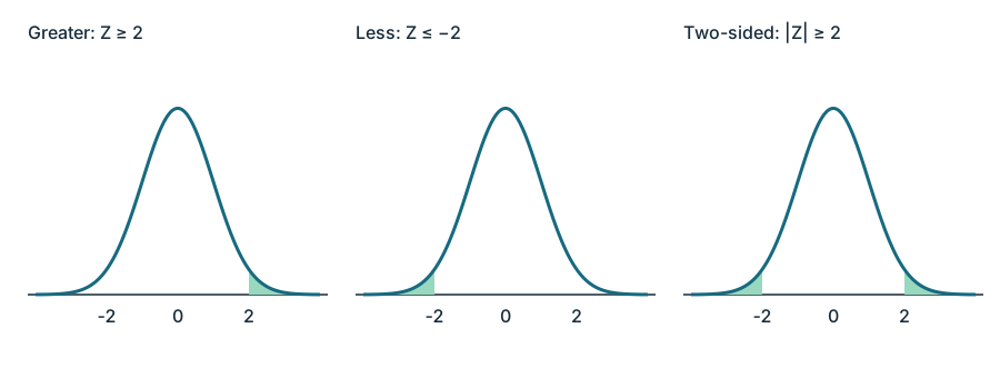
Simulation gives the same idea in counts. Generate many same-size samples under the null parameter, calculate the statistic for each, and count the proportion at least as extreme. The null-generated samples are a probability model, not additional observations from the real population. If 1,000 simulated standardized statistics include 24 at or below −2 and 31 at or above 2, an observed +2 has greater-tail p≈0.031. An observed −2 with a less alternative has p≈0.024. A two-sided ±2 result uses (24+31)/1,000=0.055, including equality in both tails. Do not automatically double one simulated tail: a finite run may not be exactly symmetric. A theoretical normal curve gives 0.02275 in either single tail and 0.04550 in both. Simulation estimates fluctuate from run to run; more repetitions improve Monte Carlo precision.

Interpret the city worked example as: if the population bottle-carrying proportion really were 0.40, about 2.64% of SRSs of 160 would have a sample proportion at least 0.475. A small p-value makes the result unusual under the null and supplies evidence for the alternative; smaller values supply stronger statistical evidence. A large p-value supplies neither convincing alternative evidence nor evidence proving the null. No p-value here is the probability H₀ is true.

Make a decision, then answer the question

The significance level α is the predetermined probability of rejecting H₀ when it is true. It can be supplied or chosen by the investigator before examining results. At a prespecified α=0.05, the worked example’s p≈0.0264≤0.05 gives reject H₀. There is convincing statistical evidence that more than 40% of city residents carry a bottle. This conclusion names the population parameter, follows the alternative and uses evidence language rather than “proves.”

If the same valid study had p=0.18, p>α would give fail to reject H₀: not enough convincing evidence of a proportion above 0.40. A test can reject or fail to reject; it cannot establish that H₀ is true. Lack of evidence for a claim is different from evidence that the claim is false. A study with low power can miss a real difference. The result is statistical reasoning that answers the original investigative question; it does not report an unexplained calculator decision or assert every resident behaves the same way.

Keep the p-value and decision distinct. A p-value of 0.032 fails to reject at α=0.01 but rejects at α=0.05. The data and conditional probability have not changed. Choosing the threshold after seeing which answer is favorable no longer follows the prespecified error-rate procedure.

Independent Application

Work through each investigation before opening the separate solutions. State parameters, show calculations and connect your reasoning to the actual study.

Original generated practice for the Fall 2026 course.

Do refill stations change habits?

A city claims that 40% of its 12,000 residents carry a reusable bottle. A simple random sample of 200 residents, drawn without replacement, contains 98 bottle carriers. The investigator asks whether the population proportion is greater than 0.40 and chooses a significance level of 0.05 before collecting data. Standard normal upper-tail probabilities: P(Z≥1.50)=0.06681; P(Z≥1.645)≈0.05; P(Z≥2.00)=0.02275; P(Z≥2.59808)≈0.004687.

Part a

Choose the inference procedure, define the population parameter in context, and write the null and alternative hypotheses. Explain which claim is represented by the alternative and what is assumed while calculating the test.

Your reasoning

Part b

Justify each of the three conditions using the actual design and numbers. State whether success/failure counts use 0.40 or the observed proportion, and explain why.

Your reasoning

Part c

Calculate the sample proportion, null standard deviation of the statistic, z-statistic and p-value. Name the null distribution and describe the tail used. Explain how a theoretical model and technology/table can supply this probability.

Your reasoning

Part d

Interpret this p-value in context, make the formal decision, and answer the investigative question with appropriately limited language. Explain why this p-value is not the probability that the null hypothesis is true.

Your reasoning

Worked answer and rubric

Three questions from the same simulated null

A fair-machine model says the population red-token proportion is 0.50. A random sample of 400 independently produced tokens contains 215 red tokens, so p̂=0.5375 and the null-standardized statistic is z=1.5. A computer generates 1,000 independent samples of 400 under p=0.50. These are generated data, not additional real-machine observations. Mutually exclusive summary counts: z<−1.5:61; z=−1.5:6; −1.5<z<1.5:859; z=1.5:8; z>1.5:66. Counts sum to 1,000. Normal-model P(Z≥1.5)=P(Z≤−1.5)=0.0668072.

Part a

For Hₐ:p>0.50, estimate the p-value from the simulation, including equality. Interpret it in context and explain why the 859 central simulations are excluded.

Your reasoning

Part b

For a different observed sample with z=−1.5 and Hₐ:p<0.50, estimate the simulated p-value. Write the corresponding theoretical normal probability and compare the estimates.

Your reasoning

Part c

Return to z=1.5 and Hₐ:p≠0.50. Estimate the two-sided simulated p-value and write its theoretical probability using absolute values. Explain why doubling the simulated upper fraction need not give the exact simulated answer.

Your reasoning

Worked answer and rubric

When the evidence is not convincing

A maker says at least 60% of its 20,000 packages arrive within two days. A consumer group takes an SRS of 150 packages without replacement and observes 81 on-time deliveries. It tests whether the population on-time proportion is below 0.60, using α=0.05. A correctly calculated lower-tail normal p-value is 0.06681. A newsletter writes: “There is a 6.681% probability the maker is right, so this proves at least 60% arrive on time.”

Part a

For the maker’s at-least-60% claim, state a null hypothesis with its inequality and the consumer group’s alternative; give the equality boundary actually tested in AP Statistics. Give both other possible alternative forms for different investigative questions, naming one-sided and two-sided tests. A second maker separately claims that at most 70% of its packages arrive within two days; an investigator asks whether its population on-time proportion exceeds 70%. Define that maker’s population parameter, state the at-most null and the investigator’s alternative, and give the equality boundary used to calculate the one-sided test.

Your reasoning

Part b

Interpret 0.06681 conditionally, state the decision and a defensible contextual conclusion, and replace both incorrect newsletter claims. Explain what changing the observed p-value to a smaller value would mean for the evidence.

Your reasoning

Worked answer and rubric

Can the model be used?

Three independent projects estimate the proportion of bicycle owners in a town. A: SRS of 120 from 8,000 people, tested H₀:p=0.02. B: a voluntary online poll of 500 people, tested H₀:p=0.50. C: SRS of 180 people from a population of 1,000, without replacement, tested H₀:p=0.50. A fourth researcher has a valid one-proportion z-test with p-value 0.032 and chooses α=0.01 before sampling; another otherwise identical study used α=0.05.

Part a

For each of A, B and C, justify which z-test conditions pass and which fail with numbers or design evidence. Explain why a large sample alone cannot repair the failed condition.

Your reasoning

Part b

Explain the meaning and timing of α in the fourth study. Make the formal decision for α=0.01 and α=0.05, and explain why changing α after seeing the p-value would undermine the stated error guarantee.

Your reasoning

Worked answer and rubric