3.3 Probability Distributions
Section Overview
- Gallery 3.3.1 - Example 3.3.1
- Example 3.3.1
- Gallery 3.3.2 - Binomial Prob. on Calc
- Example 3.3.2
- Gallery 3.3.3 - Geometric Prob. on Calc
- Gallery 3.3.4 - Example 3.3.2
- Pop Quiz 3.3.1
Random Variables
What is a random variable? Let’s look at a 6-sided die. The die could land on any one of its six faces, but we don’t know for certain which face it will land on until after we’ve made our roll. This obviously relies on probability. We have:
where:
= random variable
= specific value that the random variable takes on (in this case: 1, 2, 3, 4, 5, or 6)
The possible values that a random variables can take are determined by its probability distribution. In this section, we will learn about two common probability distributions: binomial distributions and geometric distributions.
Binomial Distribution
Binomial experiments, the experiments carried out by a binomial distribution, exhibit the following characteristics:
-
The experiment consists of a fixed number, , of identical trials.
-
Each trial results in one of two outcomes: success or failure
-
The probability of success on a single trial is equal to some value and remains the same from trial to trial. The probability of a failure is equal to .
-
The trials are independent.
-
A random variable is said to have a binomial distribution based on trials with success probability if and only if:
where
= number of trials
= number of successes
= probability of success
In general, if the random variable follows the binomial distribution with parameters and , we write . Remember not to mix up the order of the two parameters!
Gallery 3.3.1 Example 3.3.1
Frame 1 of 3
The red histogram bars represent the probability that exactly 14 applicants be accepted from part (a) Open full-size image S0239Frame 2 of 3
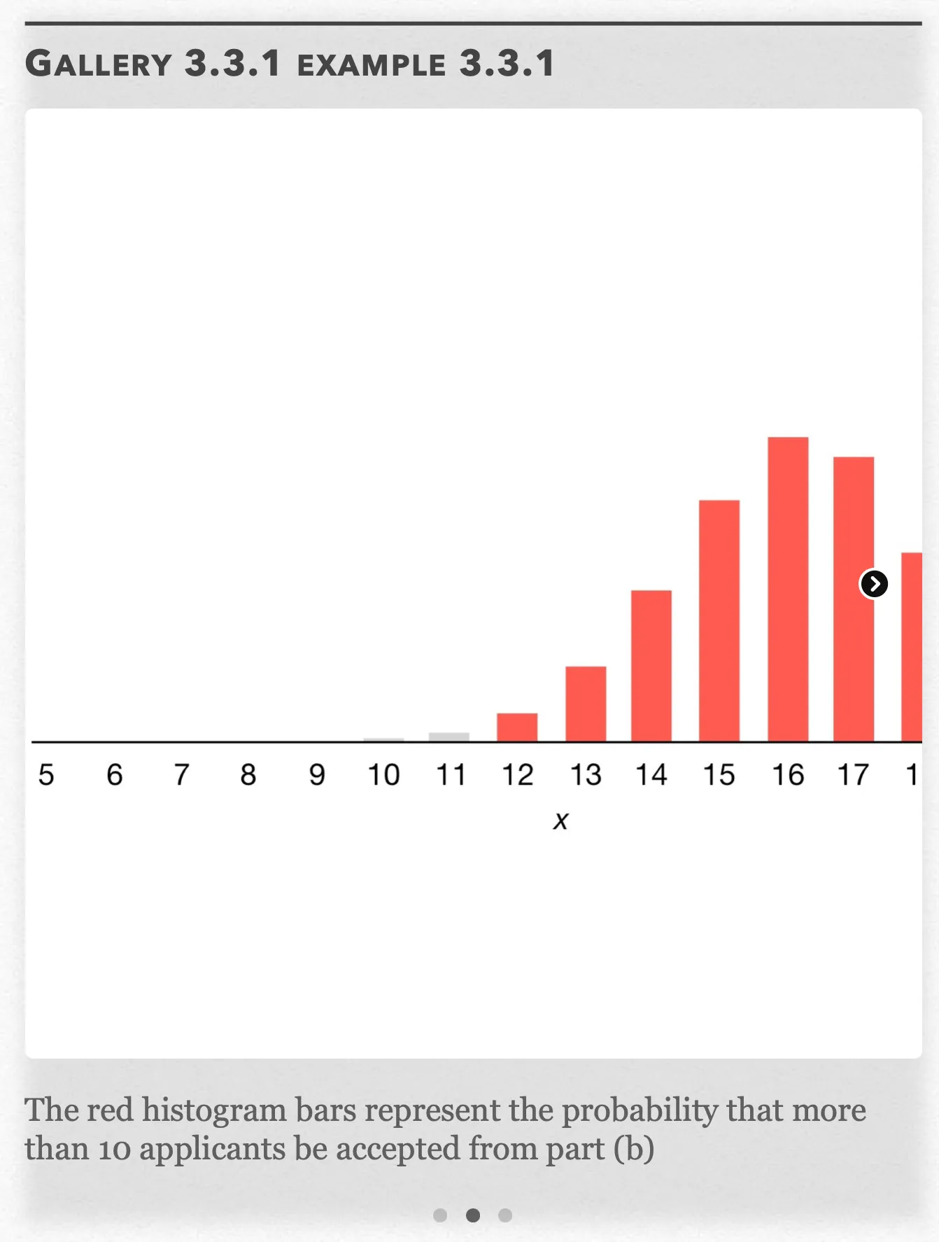
The red histogram bars represent the probability that more than 10 applicants be accepted from part (b) Open full-size image S0240Frame 3 of 3
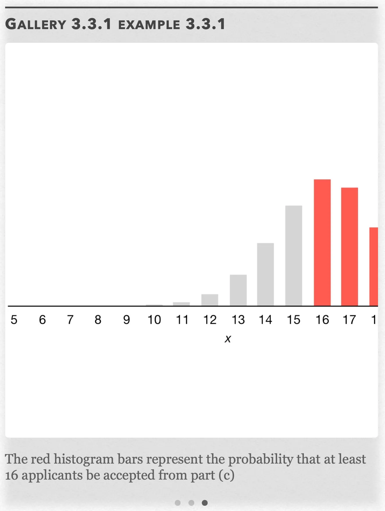
The red histogram bars represent the probability that at least 16 applicants be accepted from part (c) Open full-size image S0241
Capture provenance
Filename capture times, with no recorded timezone. Frames above follow the original gallery positions.
- · S0239 · displayed frame 1
Screenshot 2026-10-05 at 3.53.17 PM.png - · S0240 · displayed frame 2
Screenshot 2026-10-05 at 3.53.21 PM.png - · S0241 · displayed frame 3
Screenshot 2026-10-05 at 3.53.25 PM.png
Example 3.3.1 — recorded answer, introduction and part a
We are given the following information:
Let
We have 20 applicants total, so
The success probability is
The probability of success is the same for all 20 applicants, the number of applicants in the pool is a finite number, and there are only two possibilities either the applicants will be accepted or die, so we can use the binomial distribution function:
a) We need to find out the probability that exactly 14 are accepted. That is,
But we know that has binomial distribution with parameter (20, 0.8)
Gallery 3.3.2 Example 3.3.1 (Calculating binomial probabilities on TI-83/84)
Frame 1 of 3
For part (a) press 2ⁿᵈ/VARS, scroll down to “binompdf”, the binomial probability density function, and press ENTER Open full-size image S0242Frame 2 of 3
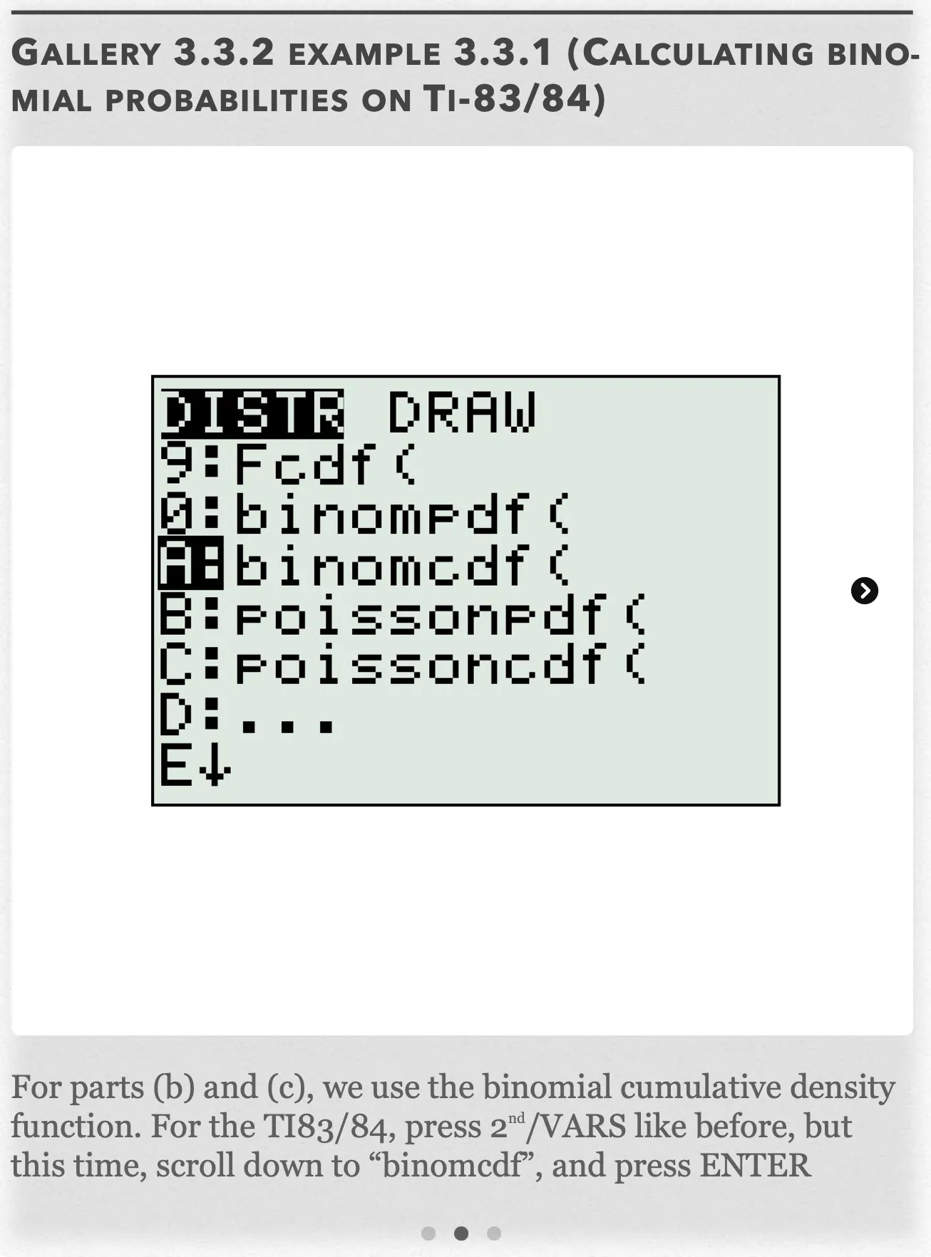
For parts (b) and (c), we use the binomial cumulative density function. For the TI83/84, press 2ⁿᵈ/VARS like before, but this time, scroll down to “binomcdf”, and press ENTER Open full-size image S0243Frame 3 of 3
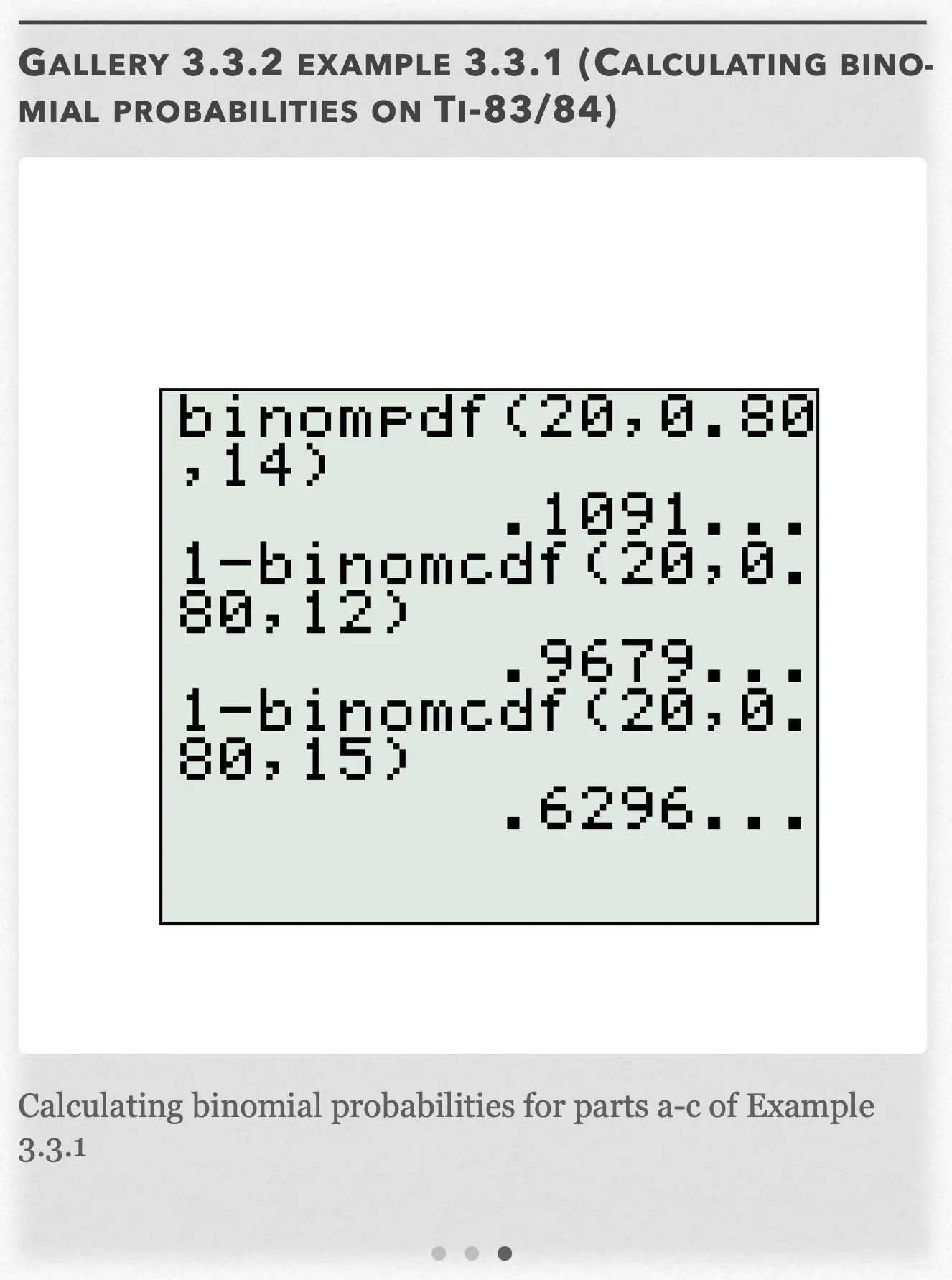
Calculating binomial probabilities for parts a-c of Example 3.3.1 Open full-size image S0244
Capture provenance
Filename capture times, with no recorded timezone. Frames above follow the original gallery positions.
- · S0242 · displayed frame 1
Screenshot 2026-10-05 at 3.53.28 PM.png - · S0243 · displayed frame 2
Screenshot 2026-10-05 at 3.53.32 PM.png - · S0244 · displayed frame 3
Screenshot 2026-10-05 at 3.53.36 PM.png
The displayed calculator expressions:
Example 3.3.1 — recorded answer, part c
c) If at least 16 applicants are accepted, then we calculate :
From what we know about the binomial cumulative density function from (b), we have:
We cannot easily calculate the above equation because the at the right of the equation doesn’t include the value of 16, which we need for the CDF. However, what is equivalent to “less than 16”? At most 15. Likewise, the equivalent value to “at least 16” is “more than 15”.
Rewriting our equation, and using our calculator (see Gallery 3.3.2 we get:
See Gallery 3.3.2 for how to calculate the probability on the calculator.
Example 3.3.1 — recorded answer, part b
b) If more than 12 applicants are accepted, then we calculate . We are going to use the cumulative density function this time.
The binomial cumulative density function calculates all values up to and including a given random variable. Since includes , we want to subtract from 1, which includes
From Gallery 3.3.2:
Geometric Distribution
The random variable with the geometric probability distribution is associated with an experiment that shares many characteristics of a binomial experiment. However, now the random variable represents number of the trial on which the first success occurs. A random variable is said to have a geometric distribution if and only if:
where
= number of successes
= probability of success
= probability of failure
In general, if the random variable follows the goemetric distribution with parameters , we write .
Example 3.3.2 — recorded answer
a) According to the problem, and
If exactly 3 holes are dug, then we calculate:
Using the calculator (See Gallery 3.3.4), we also get:
b) If at most 10 holes are dug, then we calculate :
The geometric cumulative density function calculates all values up to and including a given random variable. Since includes
Using the calculator (See Gallery 3.3.4), we get:
Gallery 3.3.3 Example 3.3.2 (Calculating geometric probabilities on TI-83/84)
Frame 1 of 3
For part (a) Press 2ⁿᵈ/VARS, scroll down to “geometpdf”, the geometric probability function, and press ENTER. Open full-size image S0247Frame 2 of 3
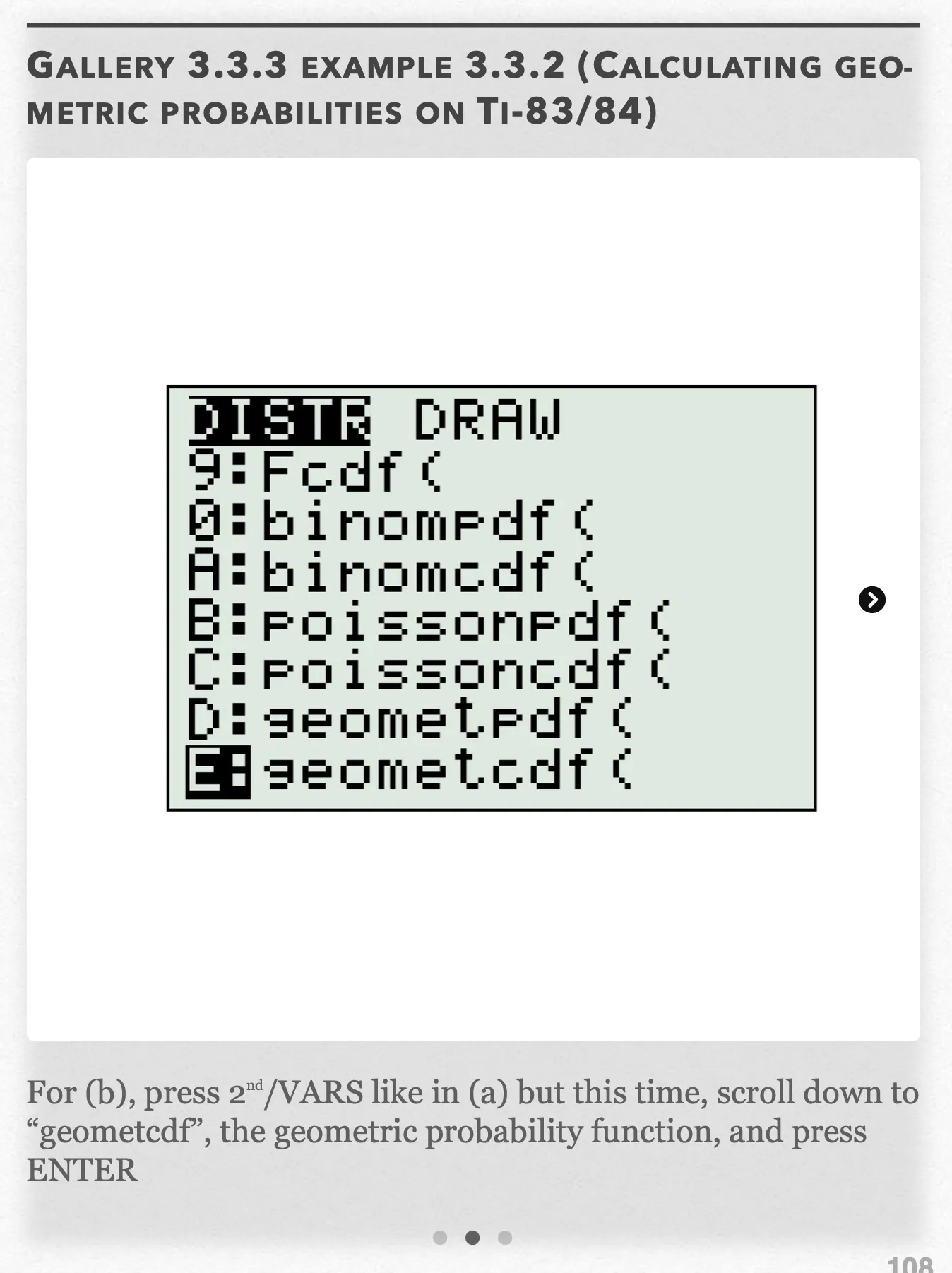
For (b), press 2ⁿᵈ/VARS like in (a) but this time, scroll down to “geometcdf”, the geometric probability function, and press ENTER Open full-size image S0248Frame 3 of 3
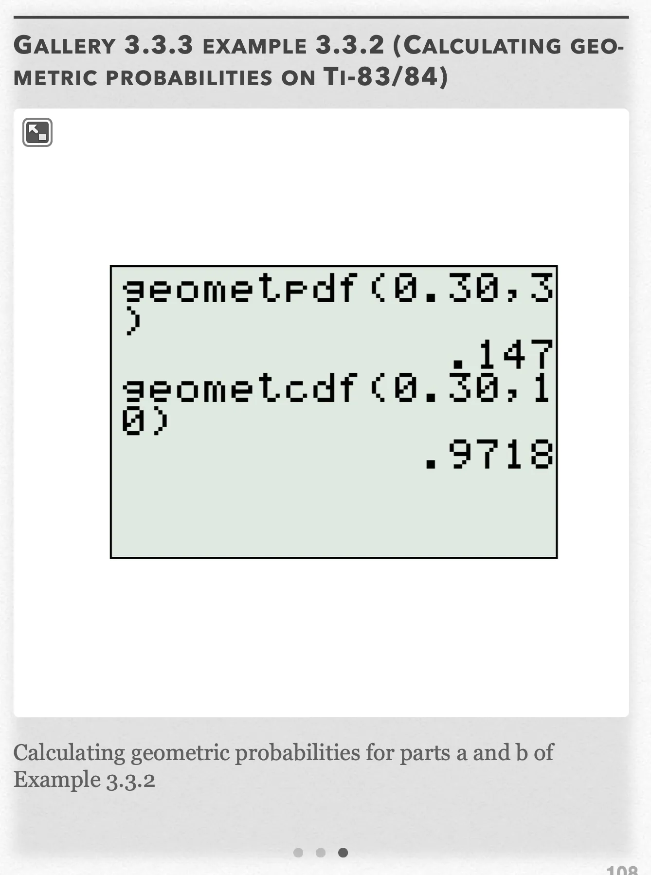
Calculating geometric probabilities for parts a and b of Example 3.3.2 Open full-size image S0249
Capture provenance
Filename capture times, with no recorded timezone. Frames above follow the original gallery positions.
- · S0247 · displayed frame 1
Screenshot 2026-10-05 at 3.53.41 PM.png - · S0248 · displayed frame 2
Screenshot 2026-10-05 at 3.53.45 PM.png - · S0249 · displayed frame 3
Screenshot 2026-10-05 at 3.53.48 PM.png
The calculator screen displays:
Gallery 3.3.4 Example 3.3.1
Frame 1 of 2
The red histogram bar represents the probability that the 3rd try will yield gold. Open full-size image S0250Frame 2 of 2
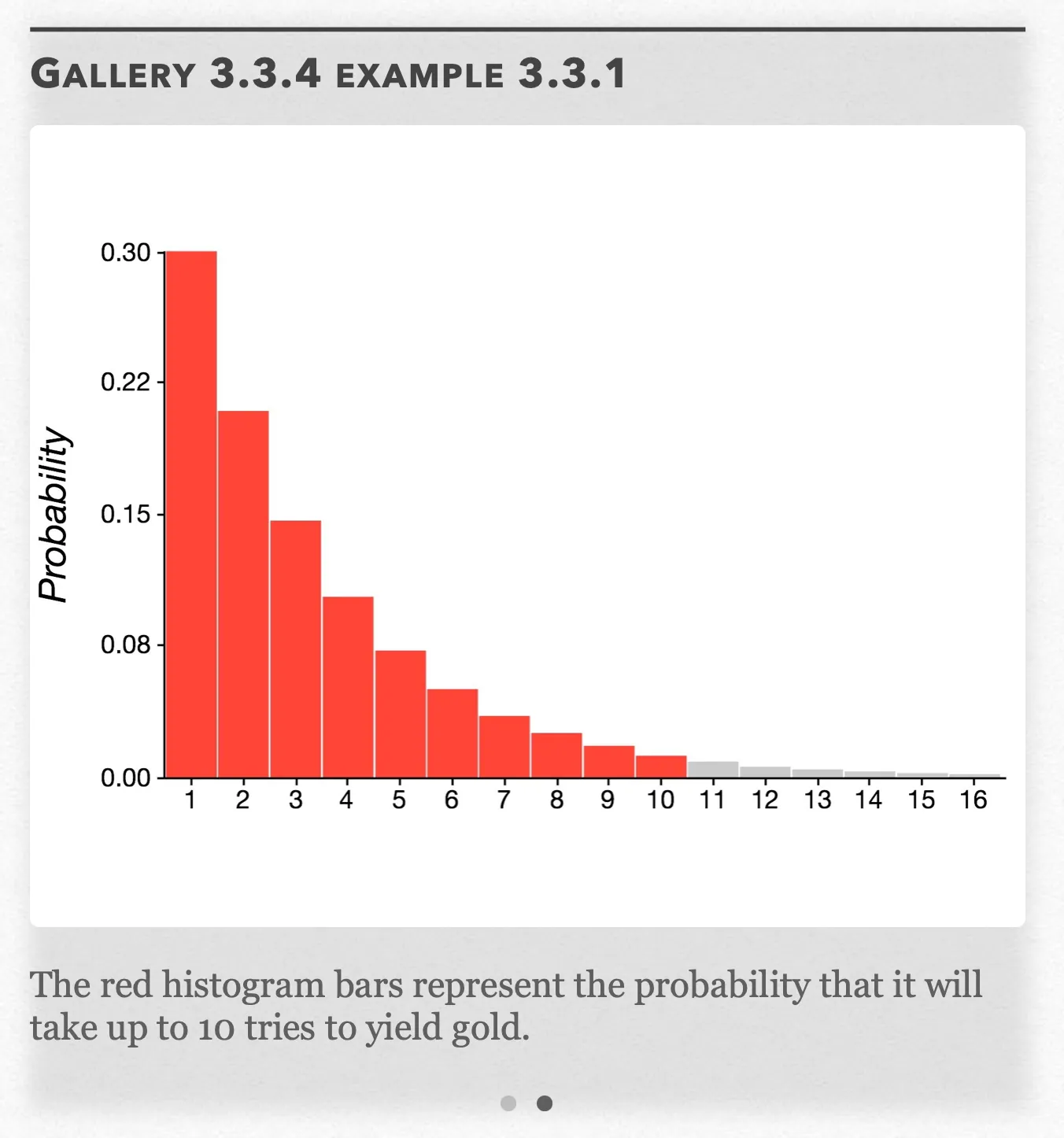
The red histogram bars represent the probability that it will take up to 10 tries to yield gold. Open full-size image S0251
Capture provenance
Filename capture times, with no recorded timezone. Frames above follow the original gallery positions.
- · S0250 · displayed frame 1
Screenshot 2026-10-05 at 3.53.50 PM.png - · S0251 · displayed frame 2
Screenshot 2026-10-05 at 3.53.54 PM.png
Expectation and Variance
We’ve learned that summary measures of a distribution include its mean and its standard deviation/variance. Random variables also have a mean (sometimes called the expected value or expectation) and variance.
The mean is the average of the values of random variable each weighted by its probability:
The variance is calculated as thus:
Both binomial and geometric distributions have a distinct expectation (or mean) and variance:
| Distribution | Mean | Variance |
|---|---|---|
| Binomial | ||
| Geometric | N/A |
Pop Quiz 3.3.1
Glossary and deeper reading · 8 refreshers
These editorial refreshers supplement the reading. Definitions and examples are added guidance; original source wording and recorded answers remain in their original context.
-
Probability
Probability quantifies how likely an event is under a specified chance model. It lies between 0 and 1, with larger values representing greater likelihood. For example, drawing a red card from a well-shuffled standard deck has probability one half.
-
Statistical independence
Statistical independence means that learning one outcome does not change the probability distribution of another. For two events, it implies that the probability of both occurring equals the product of their probabilities. For example, independent draws with replacement keep the second draw’s color probabilities unchanged by the first.
Read more: Statistical independence in the captured Statistics reading →
-
Binomial coefficient
A binomial coefficient counts the ways to select a fixed number of objects from a set when order does not matter. In a binomial probability calculation, it counts the possible success positions among the trials. For example, choosing two success positions among four trials can be done in six ways.
-
Experiment
An experiment deliberately imposes treatments and measures responses. Random assignment, comparison, and replication help distinguish treatment effects from other variation. For example, assigning plants to fertilizer treatments is an experiment.
-
Mean
The mean is a measure of center often called an average. For a finite data set, the arithmetic mean is the sum of the values divided by their number; for a random variable, the mean is its probability-weighted expected value when that value exists. Means can be pulled toward extreme values and are not generally resistant. For example, the arithmetic mean of 2, 4, and 9 is 5.
-
Standard deviation
Standard deviation measures spread around the mean using squared deviations and a square root. A sample standard deviation uses the sum of squared deviations divided by one less than the sample size before taking the square root. For example, a larger standard deviation of travel times indicates greater variability, in the original time units.
Read more: Standard deviation in the captured Statistics reading →
-
Variance
Variance is the square of the standard deviation. It measures spread in squared units, with the precise averaging rule depending on whether it describes a sample or a probability distribution. For example, a standard deviation of 3 centimeters corresponds to a variance of 9 square centimeters.
-
Expected value
Expected value is the probability-weighted mean of a random variable when that mean exists. It describes a long-run average rather than a value that must occur on one trial. For example, a fair die has expected value 3.5 even though no face is labeled 3.5.