3.4 Normal Distributions

Section Overview

Interactive 3.4.1 - Area w/ Dens. Curves
Gallery 3.4.1 - Distribution Symmetry
Interactive 3.4.2 - 67-95-99.7 Rule
Gallery 3.4.2 - z-table
Example 3.4.1
Pop Quiz 3.4.1

Density Curves

From all of the plotting methods that we’ve learned so far, the histogram comes close to resembling a density curve, which we can use to approximate the total area of the histogram bars. It is defined as a curve that:

Is always on or above the horizontal axis
Has area of exactly 1 underneath it
Represents an idealized pattern. A symmetric density curve is exactly symmetric, so the mean and median are both located dead-center. These symmetric density curves are a special class of curves, where the distribution they describe are called Normal distributions. For right-skewed density curves, the mean is greater than the median. This is because there is a greater proportion of larger values that pulls the mean away from the median. This applies in exactly the opposite way for left-skewed density curves. See Gallery 3.4.1 for a better idea.
Has mean $\mu$ (pronounced “mu”) distinguinguished from $\bar x$ , standard deviation $\sigma$ , and variance $\sigma^2$ (pronounced “sigma”) distinguished from $s_x^2$ .

Source gap (S0257): Reviewed source limitation: the original prose identifies symmetric density curves in general as Normal distributions. Symmetry alone does not establish that a distribution is Normal. The original wording is retained above.

Features of Normal Distributions

One feature that all Normal distributions with mean $\mu$ and standard deviation $\sigma$ share in common is the 68-95-99.7 Rule. It states that:

Approximately 68% of the observations fall within $\sigma$ of the mean $\mu$ .
Approximately 95% of the observations fall within $2\sigma$ of the mean $\mu$ .
Approximately 99.7% of the observations fall within $3\sigma$ of the mean $\mu$ .

This rule can be illustrated in Interactive 3.4.2

Interactive 3.4.1 Approximating Area with Density Curves

Open full-size image S0258

Source gap (S0258): The two annotation labels are visible, but their expanded explanation states are not captured.

Gallery 3.4.1 Distribution Symmetry

Frame 1 of 3

This is a symmetric distribution. The mean and the median share the same value.
Open full-size image S0259
Frame 2 of 3

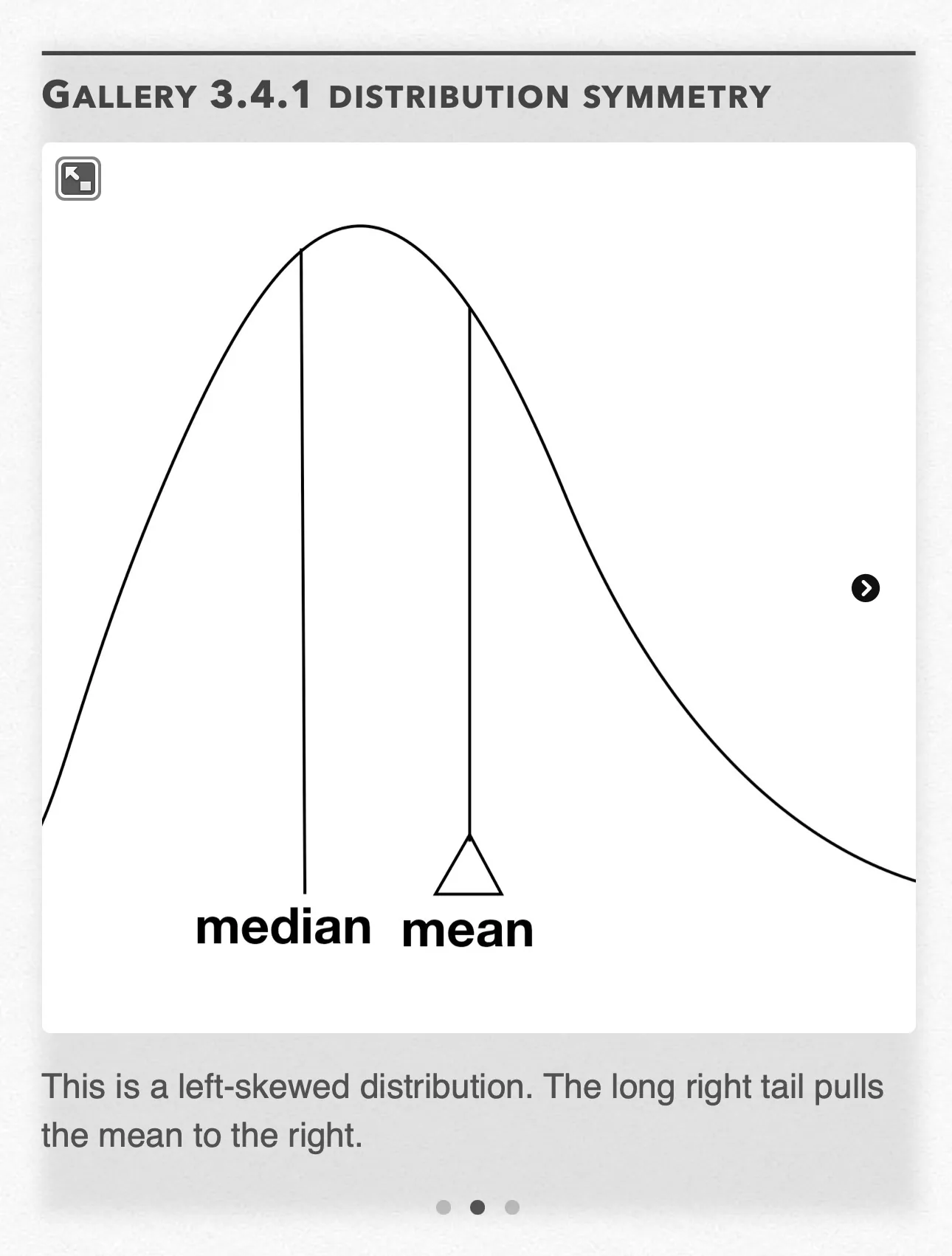
This is a left-skewed distribution. The long right tail pulls the mean to the right.
Open full-size image S0260
Frame 3 of 3

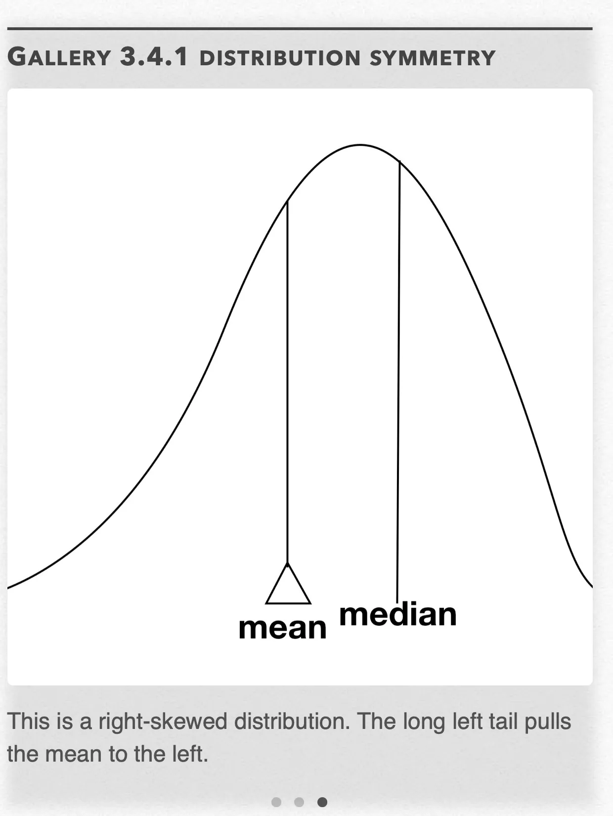
This is a right-skewed distribution. The long left tail pulls the mean to the left.
Open full-size image S0262

Capture provenance

Filename capture times, with no recorded timezone. Frames above follow the original gallery positions.

2026-10-05 15:54:12 · S0259 · displayed frame 1
Screenshot 2026-10-05 at 3.54.12 PM.png
2026-10-05 15:54:16 · S0260 · displayed frame 2
Screenshot 2026-10-05 at 3.54.16 PM.png
2026-10-05 15:54:27 · S0262 · displayed frame 3
Screenshot 2026-10-05 at 3.54.27 PM.png

Source gap (S0260): Frames 2 and 3 name the skew direction opposite the visible tail. Their original captions are retained.

Normal distributions can be standardized to what are called standard Normal distributions using the z-score formula and our “new” mean and standard deviation to find the z-score:

z=\frac{x-\mu}{\sigma}

This z-score or z-value is a value that falls on the standard Normal distribution, where it has $\mu=0$ and $\sigma=1$ . All of these z-values fall under a table called the z-table, where each z-value corresponds to a shaded “cumulative” probability up to that z-value. See Gallery 3.4.2 for a complete z-table.

Interactive 3.4.2 67-95-99.7 Rule

Open full-size image S0263

67% — recorded annotation

67% covers data that is between 1 standard deviation less than the mean and 1 standard deviation greater than the mean and is represented by the yellow region.

95% — recorded annotation

95% of the data is between 2 standard deviations less than the mean and 2 standard deviations greater than the mean and is represented by the yellow and orange regions.

99.7% — recorded annotation

99.7% of the data is between 3 standard deviations less than the mean and 3 standard deviation greater than the mean and is represented by the yellow, orange, and red regions.

Source gap (S0263): The source prose names the 68-95-99.7 Rule, while this interactive’s title, label and annotation use 67%. Both versions are retained.

Gallery 3.4.2 z-table

Frame 1 of 4

This part of the z table gives the corresponding probabilities from z=−3.49 to z=−1.75
Open full-size image S0263
Frame 2 of 4

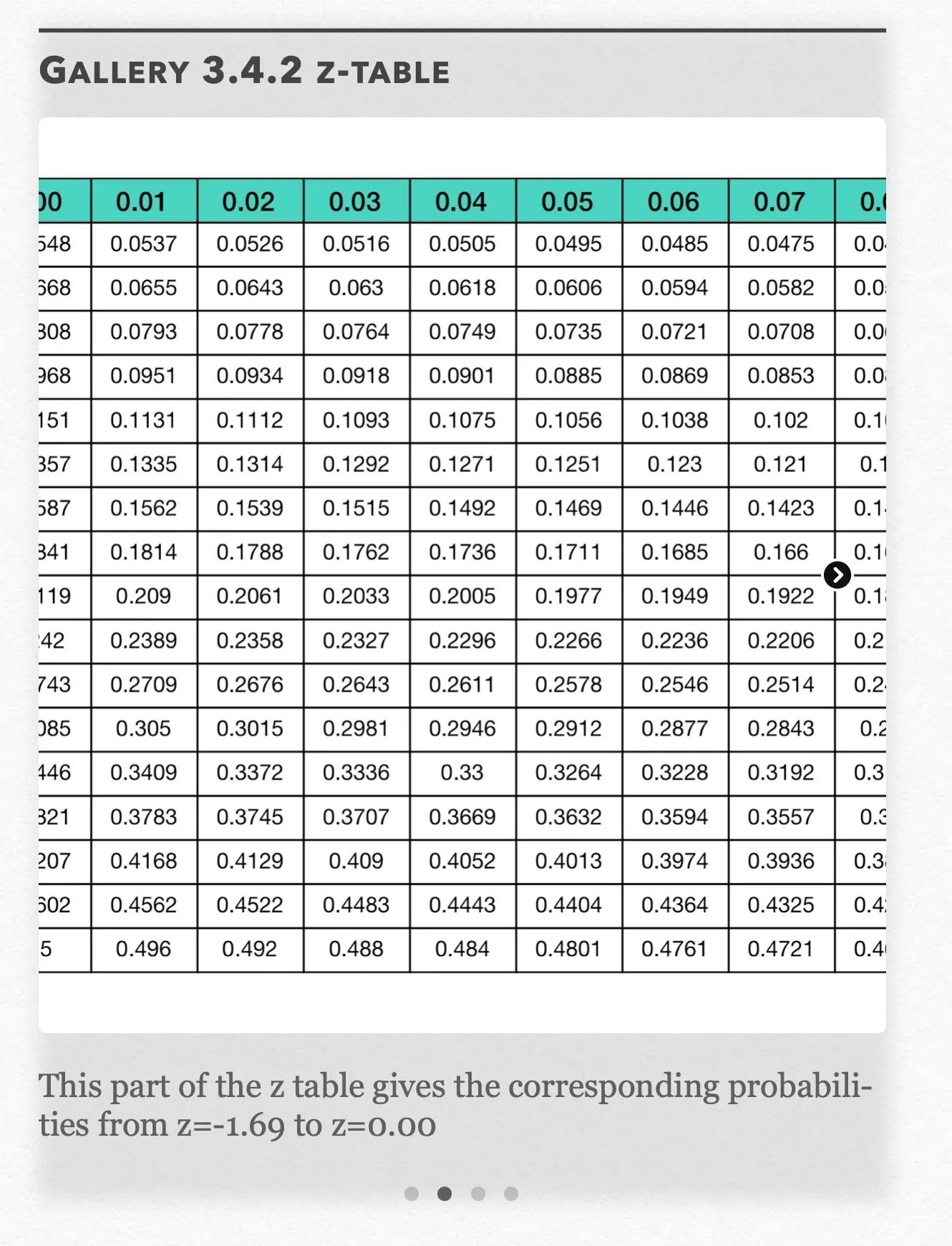
This part of the z table gives the corresponding probabilities from z=−1.69 to z=0.00
Open full-size image S0267
Frame 3 of 4

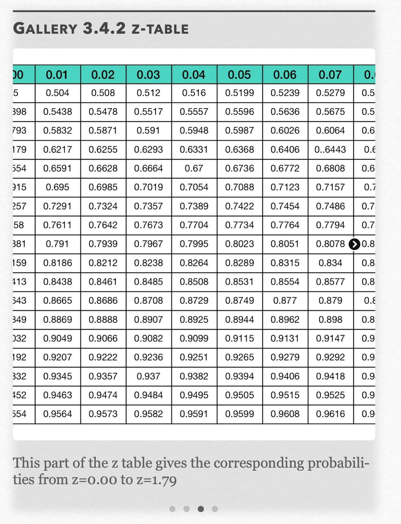
This part of the z table gives the corresponding probabilities from z=0.00 to z=1.79
Open full-size image S0268
Frame 4 of 4

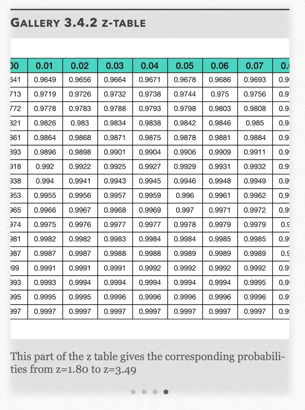
This part of the z table gives the corresponding probabilities from z=1.80 to z=3.49
Open full-size image S0269

Capture provenance

Filename capture times, with no recorded timezone. Frames above follow the original gallery positions.

2026-10-05 15:54:31 · S0263 · displayed frame 1
Screenshot 2026-10-05 at 3.54.31 PM.png
2026-10-05 15:55:04 · S0267 · displayed frame 2
Screenshot 2026-10-05 at 3.55.04 PM.png
2026-10-05 15:55:09 · S0268 · displayed frame 3
Screenshot 2026-10-05 at 3.55.09 PM.png
2026-10-05 15:55:13 · S0269 · displayed frame 4
Screenshot 2026-10-05 at 3.55.13 PM.png

Source gap (S0263): The original gallery is cropped horizontally in all four captures. Its z-value row labels, complete 0.00 column, and rightmost columns are unavailable. The following tables transfer only fully visible cells, in top-to-bottom order. “Visible row” is a transcription index, not a recovered z-value. The gallery’s original range captions are retained separately.

Gallery 3.4.2 — frame 1 visible cells

Visible row	0.01	0.02	0.03	0.04	0.05	0.06	0.07
1	0.0003	0.0003	0.0003	0.0003	0.0003	0.0003	0.0003
2	0.0005	0.0005	0.0004	0.0004	0.0004	0.0004	0.0004
3	0.0007	0.0006	0.0006	0.0006	0.0006	0.0006	0.0005
4	0.0009	0.0009	0.0009	0.0008	0.0008	0.0008	0.0008
5	0.0013	0.0013	0.0012	0.0012	0.0011	0.0011	0.0011
6	0.0018	0.0018	0.0017	0.0016	0.0016	0.0015	0.0015
7	0.0025	0.0024	0.0023	0.0023	0.0022	0.0021	0.0021
8	0.0034	0.0033	0.0032	0.0031	0.003	0.0029	0.0028
9	0.0045	0.0044	0.0043	0.0041	0.004	0.0039	0.0038
10	0.006	0.0059	0.0057	0.0055	0.0054	0.0052	0.0051
11	0.008	0.0078	0.0075	0.0073	0.0071	0.0069	0.0068
12	0.0104	0.0102	0.0099	0.0096	0.0094	0.0091	0.0089
13	0.0136	0.0132	0.0129	0.0125	0.0122	0.0119	0.0116
14	0.0174	0.017	0.0166	0.0162	0.0158	0.0154	0.015
15	0.0222	0.0217	0.0212	0.0207	0.0202	0.0197	0.0192
16	0.0281	0.0274	0.0268	0.0262	0.0256	0.025	0.0244
17	0.0351	0.0344	0.0336	0.0329	0.0322	0.0314	0.0307
18	0.0436	0.0427	0.0418	0.0409	0.0401	0.0392	0.0384

Gallery 3.4.2 — frame 2 visible cells

Visible row	0.01	0.02	0.03	0.04	0.05	0.06	0.07
1	0.0537	0.0526	0.0516	0.0505	0.0495	0.0485	0.0475
2	0.0655	0.0643	0.063	0.0618	0.0606	0.0594	0.0582
3	0.0793	0.0778	0.0764	0.0749	0.0735	0.0721	0.0708
4	0.0951	0.0934	0.0918	0.0901	0.0885	0.0869	0.0853
5	0.1131	0.1112	0.1093	0.1075	0.1056	0.1038	0.102
6	0.1335	0.1314	0.1292	0.1271	0.1251	0.123	0.121
7	0.1562	0.1539	0.1515	0.1492	0.1469	0.1446	0.1423
8	0.1814	0.1788	0.1762	0.1736	0.1711	0.1685	0.166
9	0.209	0.2061	0.2033	0.2005	0.1977	0.1949	0.1922
10	0.2389	0.2358	0.2327	0.2296	0.2266	0.2236	0.2206
11	0.2709	0.2676	0.2643	0.2611	0.2578	0.2546	0.2514
12	0.305	0.3015	0.2981	0.2946	0.2912	0.2877	0.2843
13	0.3409	0.3372	0.3336	0.33	0.3264	0.3228	0.3192
14	0.3783	0.3745	0.3707	0.3669	0.3632	0.3594	0.3557
15	0.4168	0.4129	0.409	0.4052	0.4013	0.3974	0.3936
16	0.4562	0.4522	0.4483	0.4443	0.4404	0.4364	0.4325
17	0.496	0.492	0.488	0.484	0.4801	0.4761	0.4721

Gallery 3.4.2 — frame 3 visible cells

Visible row	0.01	0.02	0.03	0.04	0.05	0.06	0.07
1	0.504	0.508	0.512	0.516	0.5199	0.5239	0.5279
2	0.5438	0.5478	0.5517	0.5557	0.5596	0.5636	0.5675
3	0.5832	0.5871	0.591	0.5948	0.5987	0.6026	0.6064
4	0.6217	0.6255	0.6293	0.6331	0.6368	0.6406	0.6443
5	0.6591	0.6628	0.6664	0.67	0.6736	0.6772	0.6808
6	0.695	0.6985	0.7019	0.7054	0.7088	0.7123	0.7157
7	0.7291	0.7324	0.7357	0.7389	0.7422	0.7454	0.7486
8	0.7611	0.7642	0.7673	0.7704	0.7734	0.7764	0.7794
9	0.791	0.7939	0.7967	0.7995	0.8023	0.8051	0.8078
10	0.8186	0.8212	0.8238	0.8264	0.8289	0.8315	0.834
11	0.8438	0.8461	0.8485	0.8508	0.8531	0.8554	0.8577
12	0.8665	0.8686	0.8708	0.8729	0.8749	0.877	0.879
13	0.8869	0.8888	0.8907	0.8925	0.8944	0.8962	0.898
14	0.9049	0.9066	0.9082	0.9099	0.9115	0.9131	0.9147
15	0.9207	0.9222	0.9236	0.9251	0.9265	0.9279	0.9292
16	0.9345	0.9357	0.937	0.9382	0.9394	0.9406	0.9418
17	0.9463	0.9474	0.9484	0.9495	0.9505	0.9515	0.9525
18	0.9564	0.9573	0.9582	0.9591	0.9599	0.9608	0.9616

Gallery 3.4.2 — frame 4 visible cells

Visible row	0.01	0.02	0.03	0.04	0.05	0.06	0.07
1	0.9649	0.9656	0.9664	0.9671	0.9678	0.9686	0.9693
2	0.9719	0.9726	0.9732	0.9738	0.9744	0.975	0.9756
3	0.9778	0.9783	0.9788	0.9793	0.9798	0.9803	0.9808
4	0.9826	0.983	0.9834	0.9838	0.9842	0.9846	0.985
5	0.9864	0.9868	0.9871	0.9875	0.9878	0.9881	0.9884
6	0.9896	0.9898	0.9901	0.9904	0.9906	0.9909	0.9911
7	0.992	0.9922	0.9925	0.9927	0.9929	0.9931	0.9932
8	0.994	0.9941	0.9943	0.9945	0.9946	0.9948	0.9949
9	0.9955	0.9956	0.9957	0.9959	0.996	0.9961	0.9962
10	0.9966	0.9967	0.9968	0.9969	0.997	0.9971	0.9972
11	0.9975	0.9976	0.9977	0.9977	0.9978	0.9979	0.9979
12	0.9982	0.9982	0.9983	0.9984	0.9984	0.9985	0.9985
13	0.9987	0.9987	0.9988	0.9988	0.9989	0.9989	0.9989
14	0.9991	0.9991	0.9991	0.9992	0.9992	0.9992	0.9992
15	0.9993	0.9994	0.9994	0.9994	0.9994	0.9994	0.9995
16	0.9995	0.9995	0.9996	0.9996	0.9996	0.9996	0.9996
17	0.9997	0.9997	0.9997	0.9997	0.9997	0.9997	0.9997

Example 3.4.1

A toy company manufactures Cuddly Critters, collectible animal plushies sold the world over. Through testing, it is found that the weight of Ulysses the Unicorn, one of the company’s most best-selling Cuddly Critters, follows a Normal distribution with mean 90 grams and standard deviation 3 grams.

a) What percent of Ulysses plushies weigh less than 85 grams?

b) What percent of Ulysses plushies weigh between 85 and 92 grams?

c) What percent of Ulysses plushies weigh more than 93.4 grams?

Example 3.4.1 — recorded answer

a) To find the percent of Ulysses plushies that weigh less than 85 grams, we have to find the corresponding z-score. Plugging in our information into the z-score formula, we get:

z=\frac{x-\mu}{\sigma}=\frac{85-90}{3}=-1.67

Using the z-table, a z-value of −1.67 corresponds to a probability of 0.0475, which is the area to the left of $z=-1.67$ on a standard normal distribution graph. This means that 4.75% of plushies weigh less than 85 grams.

b) To find the percent of Ulysses plushies that weigh between 85 and 92 grams, we have to find the corresponding z-score for both values. We already know the z-score for 85 grams is −1.67, so plugging in our information for the 92 gram value into the z-score formula, we get:

z=\frac{x-\mu}{\sigma}=\frac{92-90}{3}=0.67

Again, we already know that a z-value of −1.67 corresponds to a probability of 0.0475. Using the z-table again for 0.67, we see it corresponds to a probability of 0.7486.

We are looking for the area between $z=-1.67$ and $z=0.67$ on a standard Normal distribution graph, which we can find by calculating the difference between their corresponding probabilities:

0.7486-0.0475=0.7011

This means that 75.11% of plushies weigh between 85 grams and 92 grams.

c) To find the percent of Ulysses plushies that weigh more than 93.4 grams, we have to find the corresponding z-score. Plugging in our information into the z-score formula, we get:

z=\frac{x-\mu}{\sigma}=\frac{93.4-90}{3}=1.13

Using the z-table, a z-value of 1.13 corresponds to a probability of 0.8758, which is the area to the left of $z=1.13$ on a standard normal distribution graph. However, we want to know the percent of plushies that weigh more than 93.4 grams, which is the area to the right of $z=1.13$ . We can find this probability by subtracting 0.8758 from 1:

1-0.8708=0.1292

This means that 12.92% of plushies weigh more than 93.4 grams.

Source gap (S0271): Original inconsistencies: the difference 0.7011 is described as 75.11%; part c names 0.8758 and then subtracts 0.8708. The source’s numbers, statements and gallery captions are retained.

Gallery 3.4.3 Example 3.4.1

Frame 1 of 3

In part (a), a z-value of −1.67 means that 4.75% of plushies weigh less than 85 grams.
Open full-size image S0272
Frame 2 of 3

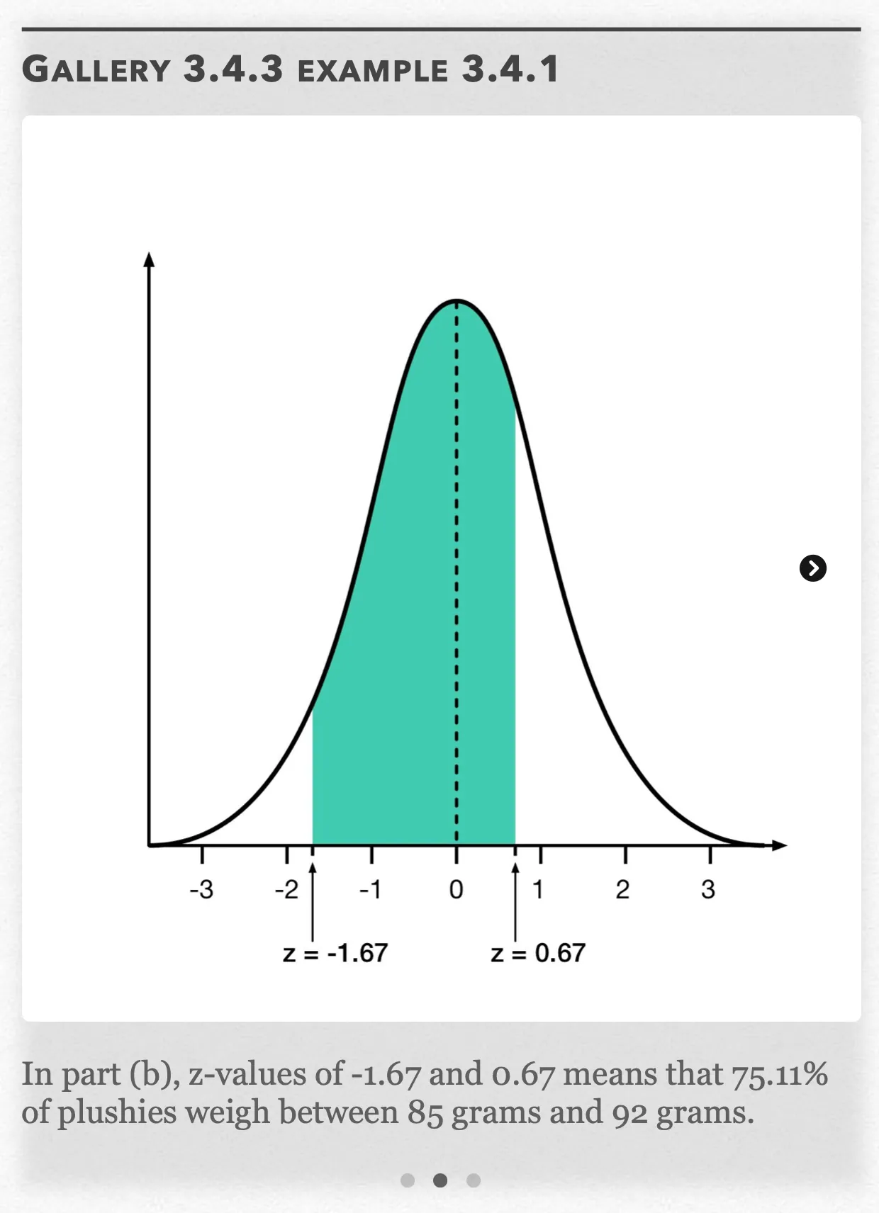
In part (b), z-values of −1.67 and 0.67 means that 75.11% of plushies weigh between 85 grams and 92 grams.
Open full-size image S0273
Frame 3 of 3

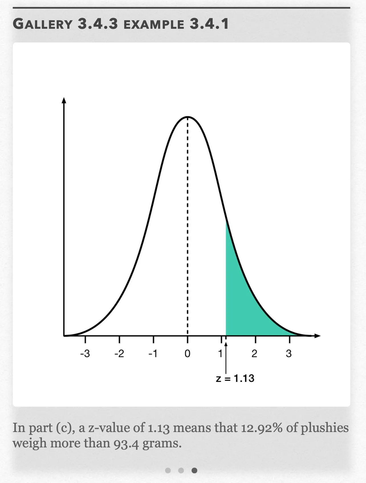
In part (c), a z-value of 1.13 means that 12.92% of plushies weigh more than 93.4 grams.
Open full-size image S0274

Capture provenance

Filename capture times, with no recorded timezone. Frames above follow the original gallery positions.

2026-10-05 15:55:22 · S0272 · displayed frame 1
Screenshot 2026-10-05 at 3.55.22 PM.png
2026-10-05 15:55:27 · S0273 · displayed frame 2
Screenshot 2026-10-05 at 3.55.27 PM.png
2026-10-05 15:55:31 · S0274 · displayed frame 3
Screenshot 2026-10-05 at 3.55.31 PM.png

Pop Quiz 3.4.1

Question 1 of 5

Which one of the following variables CANNOT possibly have a normal distribution?

A. Number of people with an A+ blood typeB. Heights of 10-year-old female childrenC. Hand spans of adult malesD. Ounces of peanut butter in cans labeled as having 12 ounces

Question 2 of 5

Pulse rates of adults are approximately Normal with a mean of 80 and a standard deviation of 5. How do we find the proportion of adults that have a pulse rate greater than 85?

A. Find the area to the left of z = 1 under a standard Normal curve.B. Find the area between z = −1 and z = 1 under a standard Normal curve.C. Find the area to the right of z = 1 under a standard Normal curve.D. Find the area to the right of z = −1 under a standard normal curve.

Question 3 of 5

If point 4 is the mean at $\mu=40$ and each point is $\sigma=2$ away from the others, then point 7 on this Normal curve corresponds to:

Open full-size image S0277

A. 43B. 46C. 47D. 50

Question 4 of 5

From question 1, what percent of the observations are between point 3 and point 6?

A. 16%B. 67%C. 81%D. 95%

Question 5 of 5

From question 1, what percent of the observations are less than point 2?

A. 1.4%B. 2.7%C. 12.4%D. 34%

Source gap (S0278): Questions 4 and 5 refer to “question 1” in the original, while the numbered-point graph appears in question 3. These references are retained. The question 3 choices wrap across lines in the screenshot but read 43, 46, 47 and 50. No checked answer feedback is captured for any of the five questions.

Glossary and deeper reading · 8 refreshers

These editorial refreshers supplement the reading. Definitions and examples are added guidance; original source wording and recorded answers remain in their original context.

Histogram
A histogram groups quantitative observations into numerical intervals and displays their frequencies or proportions. Neighboring bars represent adjacent intervals, so the graph preserves numerical order. For example, a histogram can group travel times into ten-minute intervals.
Read more: Histogram in the captured Statistics reading →
Density curve
A density curve models a continuous distribution with nonnegative height and total area 1. Probability over an interval is the area under the curve across that interval, rather than its height at a single point. For example, an interval containing one quarter of the total area has probability 0.25.
Symmetric distribution
A symmetric distribution has approximately matching shapes on either side of its center. Symmetry alone does not establish that a distribution is Normal. For example, a uniform distribution over a centered interval is symmetric but has a flat rather than bell-shaped density.
Read more: Symmetric distribution in the captured Statistics reading →
Mean
The mean is a measure of center often called an average. For a finite data set, the arithmetic mean is the sum of the values divided by their number; for a random variable, the mean is its probability-weighted expected value when that value exists. Means can be pulled toward extreme values and are not generally resistant. For example, the arithmetic mean of 2, 4, and 9 is 5.
Read more: Mean in the captured Statistics reading →
Standard deviation
Standard deviation measures spread around the mean using squared deviations and a square root. A sample standard deviation uses the sum of squared deviations divided by one less than the sample size before taking the square root. For example, a larger standard deviation of travel times indicates greater variability, in the original time units.
Read more: Standard deviation in the captured Statistics reading →
Variance
Variance is the square of the standard deviation. It measures spread in squared units, with the precise averaging rule depending on whether it describes a sample or a probability distribution. For example, a standard deviation of 3 centimeters corresponds to a variance of 9 square centimeters.
Read more: Variance in the captured Statistics reading →
68–95–99.7 rule
For a Normal distribution, approximately 68%, 95%, and 99.7% of values lie within one, two, and three standard deviations of the mean. The rule is an approximation for Normal or sufficiently bell-shaped data, rather than for every distribution. For example, a Normal model with mean 50 and standard deviation 5 places about 95% of values between 40 and 60.
Observation
An observation is a recorded value or set of values for an individual or occasion. The individual may be a person, object, or event rather than a human subject. For example, one plant’s measured height is an observation in a plant-growth study.
Read more: Observation in the captured Statistics reading →

Section Overview

Density Curves

Features of Normal Distributions

Interactive 3.4.1 Approximating Area with Density Curves

Gallery 3.4.1 Distribution Symmetry

Interactive 3.4.2 67-95-99.7 Rule

Gallery 3.4.2 z-table

Gallery 3.4.2 — frame 1 visible cells

Gallery 3.4.2 — frame 2 visible cells

Gallery 3.4.2 — frame 3 visible cells

Gallery 3.4.2 — frame 4 visible cells

Gallery 3.4.3 Example 3.4.1

Pop Quiz 3.4.1

Histogram

Density curve

Symmetric distribution

Mean

Standard deviation

Variance

68–95–99.7 rule

Observation

Help us improve Omniguides