Fall 2026 Rehearsal — Free-Response Worked Answers and Rubrics
Using the analytical rubrics
These worked solutions and task-specific rubrics accompany the separate original generated Section II rehearsal. Each question has ten independently specified points. The rubrics identify the calculation, construction, design decision, or contextual reasoning needed for credit; they are not official College Board scoring guidelines.
Credit an explicitly stated equivalent parameter order when its hypothesis, sign, tail, and conclusion remain consistent. Accept reasonable rounding and the task-specific alternatives named below. A numerical slip does not automatically remove every later point: credit later reasoning that correctly follows an identifiable earlier value when it still carries out the intended statistical action. Do not give a point for a contradictory assertion, a wrong model, an unsupported condition, or an interpretation of the wrong population quantity merely because a final number resembles the key. A correct numerical value without work can earn a point specifically for that value, but not a separate point requiring the method or explanation.
The optional practice composite is 50 times the fraction of 42 MCQs answered correctly plus 50 times the fraction of 40 FRQ points earned. It is a rehearsal percentage, not an AP score conversion or prediction. Use the rubric to plan another independent attempt after repairing a gap; it does not certify mastery by itself.
Original generated practice for the Fall 2026 course. Return to the lesson and independent checks.
1. Mulch, sunlight, and water use: worked answer
A community garden wants to investigate whether a new mulch reduces the mean weekly volume of irrigation water needed by tomato plants. Owners of 120 garden plots volunteer. Each plot contains the same tomato cultivar. Sixty plots receive full sun, and sixty receive partial shade. Sun exposure is expected to affect water use.
The two treatments are new mulch and standard mulch. Both are permitted for food gardening. Over four weeks, technicians will follow the same soil-moisture target and record the liters of irrigation water supplied to each plot each week. The response for each plot will be its mean weekly irrigation volume, in liters. The owners permit either mulch to be used.
Part a
Write a valid investigative question for this experiment. State the response, the direction of the treatment comparison, and the population or scope for which a causal conclusion would be appropriate.
One valid question is: Does using the new mulch rather than standard mulch reduce the population mean weekly irrigation volume, in liters, for tomato plots similar to these volunteer plots under the specified four-week moisture protocol? This identifies the response and a lower-mean directional comparison. Random assignment can support a causal comparison for similar plots; volunteer recruitment does not make these plots representative of all gardens.
Accept a question phrased in terms of mean(new)−mean(standard)<0, or the equivalent mean(standard)−mean(new)>0, with the response and scope clear. A question about which mulch every plant prefers or about an unmeasured outcome is not equivalent.
| Evidence for credit | Points |
|---|---|
| States mean weekly irrigation volume in liters and asks whether new mulch reduces that mean relative to standard mulch. | 1 |
| States an appropriate population of similar volunteer plots and a causal comparison under random assignment; does not generalize to all gardens from volunteer recruitment. | 1 |
Part b
Describe a randomized block design using all 120 plots. Explain why the blocks are appropriate. Give an operational random assignment procedure, the number of plots receiving each treatment in each block, and at least two concrete controls for the way water use will be measured or the plots maintained.
Use full-sun and partial-shade plots as the two blocks. Within the 60 full-sun plots, label plots 01–60 and use a random-number generator to select 30 distinct labels for new mulch; the other 30 receive standard mulch. Independently repeat the procedure within the 60 partial-shade plots. There are 30 replicates per treatment in each block, and 60 plots per treatment overall. Compare the mean water use of the two treatments within each sun block before summarizing the treatment effect.
Blocking is appropriate because sunlight affects evaporation and water use. Comparing both mulches at each sunlight level separates this known source of variation from the mulch effect and can improve precision. Do not make sunlight itself the mulch assignment.
Use the same moisture target, calibrated irrigation-volume measurement, observation schedule, cultivar, and mulch application depth wherever applicable. Give technicians a fixed watering protocol and code treatment records so the person recording volumes can be unaware of the mulch code if feasible. Other reproducible direct controls are acceptable. A claim that random assignment guarantees identical treatment groups is too strong.
| Evidence for credit | Points |
|---|---|
| Forms sunlight blocks and explains that sun exposure affects water use, so within-block comparisons control that source of variation. | 1 |
| Gives a reproducible chance procedure assigning exactly 30 plots to each mulch within each block, with no replacement or duplicate assignment. | 1 |
| Explains comparison of both treatments within each block and replication with multiple plots per treatment; uses all 120 plots. | 1 |
| Provides at least two concrete direct controls relevant to the moisture target, irrigation measurement, schedule, cultivar, or application; merely saying “keep everything the same” is insufficient. | 1 |
Part c
A gardener proposes assigning new mulch to every full-sun plot and standard mulch to every partial-shade plot. Explain the specific problem with this plan and why even a large observed treatment-group difference would not isolate the effect of mulch.
Mulch type would be completely confounded with sunlight level: every new-mulch plot is sunny, while every standard-mulch plot is shaded. Sunlight can itself alter water use, so a group difference could reflect mulch, sunlight, or both. The design has no within-sunlight treatment comparison that can separate these explanations. More plots or a more precise average would not remove this structural confounding.
Accept equivalent explanations that explicitly connect sunlight both to treatment assignment and to the irrigation response. Naming “bias” without explaining this connection is insufficient.
| Evidence for credit | Points |
|---|---|
| Identifies sunlight as confounded with mulch because the two mulch groups occupy different sun levels. | 1 |
| Explains that sunlight also affects irrigation volume, so an observed difference cannot separate a mulch effect from the sunlight effect. | 1 |
Part d
Suppose your randomized design finds convincing evidence of lower mean water use with the new mulch. State the strongest appropriate conclusion and its generalization limit. Also describe one ethical safeguard for carrying out the experiment on volunteer-owned plots.
Under the common measurement protocol, the randomized comparison supports the conclusion that new mulch causes lower mean weekly irrigation use than standard mulch for tomato plots similar to those volunteered. It does not establish an effect in every plot or representation of every garden, climate, soil type, or cultivar. The volunteers were not randomly sampled from a wider garden population.
An ethical safeguard is to obtain the owners’ informed permission, explaining random allocation to either permitted mulch, the measurements, and how any plant-health concern will be addressed. Protect identifying plot/owner information in public reports. Either a concrete informed-consent procedure or a concrete privacy/welfare safeguard earns the safeguard point; randomization by itself is not an ethical safeguard.
| Evidence for credit | Points |
|---|---|
| States a causal mean-water-use conclusion supported by random assignment and confines population application to similar volunteered plots, without asserting universal benefit. | 1 |
| Describes one concrete consent, privacy, or plant-welfare safeguard relevant to the volunteered plots. | 1 |
2. Museum puzzle times: worked answer
A museum records completion times for all 40 attendees in workshop A. Times are recorded to the nearest whole minute. The full frequency table is below; there are no other completion times.
| Time (minutes) | 4 | 5 | 6 | 7 | 8 | 12 |
|---|---|---|---|---|---|---|
| Number of attendees | 4 | 8 | 12 | 8 | 4 | 4 |
A separate workshop B also has 40 attendees. Its five-number summary, in minutes, is minimum 3, Q1 = 5, median = 7, Q3 = 9, maximum 11. For all quartiles in this question, use the median of the lower half and the median of the upper half of the ordered data.
Part a
Construct a labeled dotplot for workshop A, keeping the horizontal axis on an evenly spaced time scale. You may provide a drawing or complete plotting instructions giving the axis label, time locations, and number of dots at every occupied location. Do not merely name the type of graph.
Label the horizontal axis “Completion time (minutes)” with equally spaced integer positions from 4 through 12. Stack 4 dots at 4, 8 at 5, 12 at 6, 8 at 7, 4 at 8, and 4 at 12. Leave positions 9, 10, and 11 empty. Each dot represents one attendee, for a total of 40 dots.
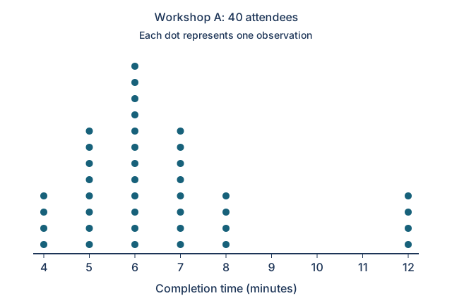
Accept horizontal rather than vertical stacking if the time axis remains evenly spaced and all 40 values are represented. Joining the six time values as evenly spaced categories would incorrectly hide the 8-to-12 gap.
| Evidence for credit | Points |
|---|---|
| Uses a labeled time axis in minutes on an evenly spaced numeric scale, preserving the empty locations 9–11. | 1 |
| Shows or specifies exactly 4, 8, 12, 8, 4, and 4 dots at times 4, 5, 6, 7, 8, and 12, for all 40 attendees. | 1 |
Part b
Calculate the mean and median completion time for workshop A. Show how the frequencies or ordered positions produce each result.
The mean is minutes. The cumulative counts are 4 through time 4, 12 through time 5, and 24 through time 6. Therefore both the 20th and 21st ordered times are 6, and the median is minutes.
Accept an equivalent expansion of all 40 times. Averaging the six distinct time labels without weighting their frequencies does not give the attendee mean.
| Evidence for credit | Points |
|---|---|
| Calculates the frequency-weighted mean as 264/40 = 6.6 minutes. | 1 |
| Uses the 20th and 21st ordered observations to obtain the median of 6 minutes. | 1 |
Part c
Calculate Q1, Q3, the IQR, and both 1.5×IQR outlier fences for workshop A. Identify all observed outlier values, if any. Values exactly on a fence are not outliers.
The lower half consists of positions 1–20; its 10th and 11th values are both 5, so Q1=5 minutes. The upper half consists of positions 21–40; the 30th and 31st overall values are both 7, so Q3=7 minutes. Thus IQR=7−5=2 minutes. The lower fence is minutes and the upper fence is minutes. All four 12-minute observations are upper outliers. There are no lower outliers because the minimum, 4, is above 2.
Use strict below/above comparisons. Neither 4 nor 8 is an outlier; the fences are cutoffs, not observed minimum and maximum values.
| Evidence for credit | Points |
|---|---|
| Obtains Q1=5, Q3=7, IQR=2 and both fences 2 and 10 minutes with a valid calculation. | 1 |
| Identifies the four 12-minute observations as the only outliers, and explicitly rules out lower outliers. | 1 |
Part d
Compare typical completion time and the variability of the middle half of attendees in workshops A and B, using the median and IQR. Explain why those two statistics are useful for workshop A.
The median is lower in A (6 minutes) than in B (7 minutes), so a typical attendee finishes about 1 minute sooner in A by the median. The IQR is 2 minutes in A and 9−5=4 minutes in B, so A’s middle half is less variable. The 12-minute outliers in A can pull the mean and standard deviation upward; the median and IQR are resistant to those extreme times and describe the main group more stably.
Do not infer that every A attendee is faster or that workshop membership causes the difference. The question describes these two workshop groups rather than a randomized treatment comparison.
| Evidence for credit | Points |
|---|---|
| Compares both medians in context (A 6 versus B 7 minutes) and both IQRs (A 2 versus B 4 minutes), with correct direction. | 1 |
| Justifies median/IQR for A by their resistance to the observed upper outliers, contrasted with mean/SD sensitivity. | 1 |
Part e
One of workshop A’s 40 attendees is chosen uniformly at random. Calculate the probability that the attendee’s completion time is at least 8 minutes. Also calculate the percentile rank of a 6-minute completion time, using the percentage of times less than or equal to 6.
There are 4 attendees at 8 minutes and 4 at 12, so . There are times at or below 6, giving , or the 60th percentile under the stated at-or-below convention. Including all 12 ties at 6 is essential here; counting only strictly smaller times would give 30%, which answers a different question.
| Evidence for credit | Points |
|---|---|
| Calculates the at-least-8-minute event as 8/40 = 0.20, including both 8 and 12 minutes. | 1 |
| Calculates the 6-minute at-or-below percentile as 24/40 = 60%, including all ties at 6. | 1 |
3. Comparing two route-planning methods: worked answer
A delivery depot wants to determine whether a new route-planning method lowers mean driving time relative to its old method. A simple random sample of 20 drivers is selected without replacement from the depot’s 6,000 drivers. Each selected driver completes one comparable route using each method; the order of the methods is randomized independently for each driver. Routes have the same distance and stop schedule within each driver’s comparison, and the study conditions are otherwise held constant. Assume results from different drivers can be treated as independent.
For each driver, define d = old-method driving time − new-method driving time, in minutes. For the 20 differences, the sample mean is 4.6 minutes and the sample standard deviation is 7.2 minutes. The distribution of differences is roughly symmetric with no outliers. The population SD of differences is unknown. Use α = 0.05.
| Positive t cutoff | Upper-tail probability |
|---|---|
| 1.729 | 0.05 |
| 2.539 | 0.01 |
| 2.861 | 0.005 |
| 3.174 | 0.0025 |
You may use technology for a p-value or give a correct bound using this table.
Part a
Define the population parameter and state the null and alternative hypotheses for whether the new method lowers mean driving time.
Let be the population mean old-minus-new driving-time difference, in minutes, for drivers at this depot under the comparable-route protocol. A reduction by the new method corresponds to a positive old-minus-new difference. Test against .
Accept an explicitly reversed new-minus-old parameter with a less-than alternative if every later sign and tail is consistent. Hypotheses must concern the population mean difference, not the observed sample mean 4.6.
| Evidence for credit | Points |
|---|---|
| Defines a population mean within-driver driving-time difference for depot drivers, with subtraction order and minutes clear. | 1 |
| States equality to zero under H0 and a correctly directed alternative for lower new-method time, consistent with the chosen order. | 1 |
Part b
Identify the appropriate inference procedure and its degrees of freedom. Justify it by verifying the randomization, sampling-fraction, and sample-shape conditions using the information given.
Use a paired t-test, equivalently a one-sample t-test on the 20 old-minus-new differences, with df=20−1=19. The same drivers receive both methods, so there is one sample of paired differences rather than two independent samples of driving times.
The drivers were selected by a simple random sample, and method order was randomized. For without-replacement sampling, 20 is less than 10% of 6,000 (=600). Because n=20<30, examine the distribution of differences: it is roughly symmetric and free of outliers, supporting the t procedure. Check the differences, not separate old/new marginal distributions. The context supplies independence between drivers.
| Evidence for credit | Points |
|---|---|
| Selects a one-sample t-test on paired differences with df=19 and explains the same-driver pairing. | 1 |
| Uses the random selection/order information and verifies 20≤600 for the 10% condition. | 1 |
| Uses the roughly symmetric, outlier-free distribution of differences for n=20; does not claim n≥30. | 1 |
Part c
Calculate the standard error and test statistic. Obtain the appropriately directed p-value or a correct bound, showing enough work to identify the reference distribution and tail.
The standard error is minutes. The test statistic is . For a t-distribution with 19 degrees of freedom, . This is one upper tail, because the alternative is .
Using the supplied rounded table, the observed t lies between 2.539 and 2.861, so is an acceptable bound. Accept a correctly reversed sign and lower tail for a reversed parameter. Doubling the tail would answer a two-sided alternative instead.
| Evidence for credit | Points |
|---|---|
| Computes s_d/sqrt(20) ≈ 1.610 minutes for the standard error. | 1 |
| Computes the signed t statistic ≈ 2.857 with null difference zero and the correct denominator. | 1 |
| Uses a one-sided t19 tail to obtain approximately 0.00504 or the valid bound 0.005<p<0.01. | 1 |
Part d
Make the decision at α = 0.05 and state a conclusion about the population in context. Avoid wording that proves a hypothesis or promises a decrease for every driver.
Because p≈0.00504<0.05 (and the table bound is also entirely below 0.05), reject H0. There is convincing statistical evidence that the population mean old-minus-new driving-time difference is positive for drivers at this depot under the comparable-route protocol. Equivalently, the new method lowers mean driving time under these study conditions.
The SRS supports generalization to depot drivers; it does not represent drivers at every other depot. Randomized method order and the controlled paired routes support a treatment comparison under the protocol. The result concerns an average and neither proves the parameter’s exact value nor guarantees a decrease for every driver. A conclusion following a correctly reversed definition is equivalent.
| Evidence for credit | Points |
|---|---|
| Explicitly compares p or its correct bound with 0.05 and rejects H0. | 1 |
| States convincing evidence of lower population mean new-method time for the depot-driver protocol, using non-definitive language and the correct mean/difference direction. | 1 |
4. Parcel times and dispatch delays: worked answer
Two parcel depots, A and B, each served more than 20,000 different customers last month. For this question, every customer placed exactly one order during that month. A researcher independently takes a simple random sample of 100 customers from each depot’s customer list, without replacement, and records elapsed time from order to delivery, in days. Assume sampled customer responses can be treated as independent within each sample, and the two depot samples are independent.
| Delivery time (days) | 1 | 2 | 3 | 4 | 5 |
|---|---|---|---|---|---|
| Number of sampled customers | 10 | 20 | 40 | 20 | 10 |
For A, the sample standard deviation is 1.101 days (rounded). For B, the sample mean is 3.6 days and the sample standard deviation is 1.4 days (rounded). The B sample has no strong skewness or outliers. Neither population SD is known. A technology calculation for a 90% two-sample t-interval gives df≈187.6 and t*≈1.653; use that critical value.
Separately, for 40 parcels from depot A, a researcher records x = hours between order and dispatch and y = days between order and delivery. The observed x values range from 4 through 40 hours. A scatterplot supports a linear model, with no influential outliers. The fitted line is , and r=0.75. One parcel has x=25 hours and observed y=4 days.
Part a
Identify the appropriate procedure to estimate μA−μB, the difference in population mean delivery time for A minus B. Explain why these samples are independent rather than paired, and verify the conditions for the procedure using the given design, population sizes, and sample information.
Use a two-sample t-interval for the difference between population mean delivery times, A minus B. The researcher samples distinct customer populations independently; there is no matching of an A customer to a B customer and no repeated treatment on the same customer.
Both samples are simple random samples and independent. Each sample of 100 is less than 10% of its population of more than 20,000. Both sample sizes are at least 30; A’s bounded symmetric frequency distribution and B’s stated absence of strong skewness/outliers further support the approximation. Unknown population SDs require estimated standard errors and t inference.
Calling the samples paired solely because both have 100 customers is a material design error. A one-mean procedure estimates a different parameter.
| Evidence for credit | Points |
|---|---|
| Identifies a two-sample t-interval for A-minus-B population means and explains independent customer samples rather than pairing. | 1 |
| Verifies random/independent sampling, the separate 10% bounds, and both n=100 sample-shape/sample-size conditions using actual context. | 1 |
Part b
A sampled depot-A customer is selected uniformly at random. Calculate the probability that this customer’s order took at most 2 days. Calculate the sample mean delivery time for A from the complete frequency table.
The at-most-2-day event includes the 10 one-day and 20 two-day deliveries: . The sample mean is days. Both calculations use the 100 customer observations, not the five distinct time labels as equally likely outcomes.
The 0.30 is a descriptive probability for selecting from this finite sample, not the exact unknown population probability.
| Evidence for credit | Points |
|---|---|
| Calculates (10+20)/100=0.30 for at most 2 days, including the equality boundary. | 1 |
| Calculates the frequency-weighted mean as 300/100=3.0 days. | 1 |
Part c
Calculate a 90% confidence interval for μA−μB using the supplied critical value. Interpret it in context and state whether it gives convincing evidence of a difference in population mean delivery times.
The point estimate is day. The estimated standard error is day. The margin of error is day. Thus the 90% interval is , or approximately day.
We are 90% confident that depot A’s population mean delivery time is between 0.3056 and 0.8944 day shorter than depot B’s, for the defined customers and orders from last month. Since every plausible A-minus-B mean difference in this interval is negative and zero is excluded, the interval provides convincing evidence that A’s population mean delivery time is lower. This observational comparison of depots does not establish that moving an order to A causes the improvement.
Accept equivalent A-minus-B interpretations with endpoints rounded reasonably, or an explicitly reversed B-minus-A interval and direction. Using the exact A SD from the frequency table changes the displayed endpoints negligibly. A conservative df=99 calculation gives a slightly wider interval and is acceptable if the alternative critical value and method are explicitly justified. Do not describe the endpoints as containing 90% of individual delivery times.
| Evidence for credit | Points |
|---|---|
| Computes the difference −0.6 and the unpooled standard error about 0.1781 using both s²/n terms. | 1 |
| Uses the supplied t critical value to obtain approximately (−0.8944,−0.3056) day, or a justified equivalent t interval with reasonable rounding. | 1 |
| Interprets the population mean difference with 90% confidence and concludes A is lower because zero is excluded; does not claim individual-time coverage or causality. | 1 |
Part d
For the separately modeled parcel with x=25 hours, calculate the predicted delivery time and its residual, then explain what the residual says about the prediction. Calculate r² and interpret it for this parcel regression.
The predicted time is days. Since the observed time is 4 days, the residual is day: the model underpredicts this parcel’s delivery time by 1 day. The 25-hour x value is within the observed range, so this prediction is interpolation.
The coefficient of determination is . About 56.25% of the observed variation in delivery time (the response, in days) for the 40 parcels is explained by the linear relationship with order-to-dispatch time (the explanatory variable, in hours). It does not mean that 56.25% of each parcel’s time is caused by dispatch delay, and it is not the fraction of dispatch-time variation explained by delivery time.
| Evidence for credit | Points |
|---|---|
| Calculates the predicted time as 3 days by substituting x=25 into the line. | 1 |
| Calculates residual +1 day as observed minus predicted and states that the model underpredicts by 1 day. | 1 |
| Calculates r²=0.5625 and interprets 56.25% of delivery-time variation explained by the linear relationship with dispatch time, using the correct response. | 1 |