Fall 2026 Rehearsal — Multiple-Choice Worked Answers
After an independent attempt
These worked answers explain the original generated questions in the separate Section I rehearsal. Each item earns one point for its correct choice. Read the reasoning even when your choice was correct: a matching letter can result from a lucky guess or an incorrect calculation.
For each missed item, identify the statistical quantity, repair the model or reasoning, and recompute before checking the explanation again. The two shared settings have three separate questions each; getting one correct does not settle the others. These answers are newly authored practice solutions, not recovered keys for the preserved historical test.
Original generated practice for the Fall 2026 course. Return to the lesson and independent checks.
1. Cycling commute distance: worked answer
A town has 12,000 registered cyclists. A transportation planner will randomly select 200 of them and record each cyclist’s total cycling commute distance, in miles, during a specified week. The planner wants to estimate a population mean.
Part a
Which is a valid investigative question that matches this purpose and the data to be collected?
The question identifies the quantitative variable (weekly cycling commute miles), the population (all registered cyclists in the town), and the estimation goal (an interval for the population mean). A single individual’s exact value and a total for the particular sample do not address this population-mean goal. The data do not support a universal causal claim about residents.
| Evidence for credit | Points |
|---|---|
| Select B. This item earns one point for the correct choice; the worked answer explains the reasoning. | 1 |
2. Support for a proposed walkway: worked answer
A city planner will independently select random samples of registered voters from the east and west districts. Each voter will answer the same yes/no question about support for a proposed public walkway. The planner wants to investigate whether population support differs between the districts.
Part a
Which investigative question fits the study?
The response is support (yes/no), the parameters are the two population proportions, and the question asks whether they differ. Random sampling permits population comparisons, but the planner does not assign residence, so the study cannot identify an effect of moving districts. Daily use and strength of opinion are not measured.
| Evidence for credit | Points |
|---|---|
| Select C. This item earns one point for the correct choice; the worked answer explains the reasoning. | 1 |
3. Sampling apartment buildings: worked answer
A housing agency divides its service area into 80 apartment buildings. It randomly selects 8 buildings and surveys every household in each selected building. The buildings have broadly similar mixes of household sizes.
Part a
Which sampling method is described?
The agency randomly selects whole groups (buildings) and includes every household in the selected groups, so this is cluster sampling. Stratified sampling would select households from every stratum. Not every set of the same number of households has an equal chance of selection, as it would in a household-level simple random sample. No fixed sampling interval is used.
| Evidence for credit | Points |
|---|---|
| Select D. This item earns one point for the correct choice; the worked answer explains the reasoning. | 1 |
4. A bus-service feedback poll: worked answer
A transit agency places an optional online poll on its website asking riders to rate the bus service. Only riders who choose to visit the website and submit a response are included. The agency uses the results to estimate the proportion of all riders who are dissatisfied.
Part a
Which is the clearest potential source of bias?
This is voluntary response sampling: respondents select themselves. Strongly dissatisfied riders may be more likely to submit feedback than other riders, producing a systematic overestimate of dissatisfaction. That direction is a plausible risk, not a guaranteed outcome. A large sample can reduce random variability without correcting selection bias.
| Evidence for credit | Points |
|---|---|
| Select A. This item earns one point for the correct choice; the worked answer explains the reasoning. | 1 |
5. Diet and starting age: worked answer
A researcher will compare two diets for 80 kittens. Forty kittens are 8 weeks old and forty are 16 weeks old. Starting age is expected to affect weight gain. Each kitten will receive one diet for the same period.
Part a
Which allocation best addresses the known age effect while allowing a comparison of the diets?
Blocking by starting age places similar kittens together, and random assignment of both diets within each block allows fair diet comparisons at each age. Assigning diets by age would confound diet and age. Selecting promising kittens for one diet introduces a systematic group difference, and using only one diet removes the treatment comparison.
| Evidence for credit | Points |
|---|---|
| Select C. This item earns one point for the correct choice; the worked answer explains the reasoning. | 1 |
6. Volunteers and a sleep program: worked answer
Sixty adults volunteer for a study. They are randomly assigned to a new sleep program or a control program. Procedures other than the assigned program are the same, and the new-program group has a convincingly greater average improvement in nightly sleep duration.
Part a
Which conclusion is best supported by the design?
Random assignment reduces potential confounding and supports a cause-and-effect comparison of the programs. The volunteer recruitment limits population generalization to adults similar to those studied; it does not establish representation of all adults. The conclusion concerns an average effect and does not promise benefit for every participant.
| Evidence for credit | Points |
|---|---|
| Select B. This item earns one point for the correct choice; the worked answer explains the reasoning. | 1 |
7. Sample standard deviation: worked answer
A student records the checkout times, in minutes, for four randomly selected library visits: 2, 4, 4, and 6.
Part a
What is the sample standard deviation of these four times, in minutes?
The sample mean is 4 minutes. The squared deviations sum to , so minutes. Dividing by 4 gives a population-formula value of 1.414; 2.667 is the sample variance, and 4 is the range.
| Evidence for credit | Points |
|---|---|
| Select B. This item earns one point for the correct choice; the worked answer explains the reasoning. | 1 |
8. Representing two commute modes: worked answer
A university wants to estimate mean commute time for its students. Bus commuters and rail commuters may have different travel-time distributions. A complete student list identifies each commuter’s mode. The university can contact a randomly chosen student in either group at the same cost.
Part a
Which plan is most appropriate if the university wants both commute modes represented through random selection?
A stratified random sample using commute mode ensures that both distinct groups contribute randomly selected students. The eventual overall estimate should respect the population sizes of the two strata. Convenience selection, omitting bus commuters, and voluntary response do not satisfy the stated goal.
| Evidence for credit | Points |
|---|---|
| Select D. This item earns one point for the correct choice; the worked answer explains the reasoning. | 1 |
9. Checkout-time shape: worked answer
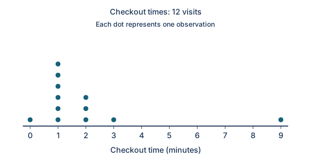
The dotplot shows checkout times, in minutes, for 12 visits. Each dot represents one visit.
Part a
Which description best fits the distribution?
The main peak is at 1 minute, and most times lie from 0 to 3 minutes. The lone 9-minute value extends the tail to the right, with no times between 3 and 9. Equal counts at the two extremes do not make the distribution symmetric, and one dot per visit does not imply equal frequencies at each time.
| Evidence for credit | Points |
|---|---|
| Select A. This item earns one point for the correct choice; the worked answer explains the reasoning. | 1 |
10. Comparing delivery routes: worked answer
| Route | Minimum | Q1 | Median | Q3 | Maximum |
|---|---|---|---|---|---|
| A | 8 | 10 | 12 | 14 | 32 |
| B | 10 | 12 | 14 | 16 | 20 |
The summaries describe two separate samples of deliveries.
Part a
Which comparison is supported by the summaries?
Route A’s median is 12 minutes, compared with 14 for B. Both IQRs are 4 minutes: 14−10 and 16−12. A’s range is 24 minutes, compared with 10 for B. A lower median indicates a lower typical time by this measure, not that every delivery on A is faster.
| Evidence for credit | Points |
|---|---|
| Select C. This item earns one point for the correct choice; the worked answer explains the reasoning. | 1 |
11. A new invitation: worked answer
Two hundred employees volunteer for a training study. They are randomly assigned, 100 per group, to receive either the standard invitation or a new invitation. Enrollment within one week is recorded as yes or no. The researcher’s goal is to determine whether the new invitation increases enrollment.
Part a
Which investigative question best includes the study’s response, direction, and defensible causal scope?
The selected question names the binary enrollment response, asks about an increase in a proportion, and uses a population of employees similar to the volunteers. Random assignment supports a causal effect of receiving the invitation. Volunteer recruitment does not support a claim about every employee or company, and merely reporting a sample proportion does not address the causal investigative purpose.
| Evidence for credit | Points |
|---|---|
| Select B. This item earns one point for the correct choice; the worked answer explains the reasoning. | 1 |
12. A conditional refund probability: worked answer
Probability set: questions 12–14. An airline has complete records for 200 passengers on one flight. A passenger will be selected uniformly at random from these 200. Let A mean that the passenger used the airline app, and let R mean that the passenger claimed a refund. The table classifies every passenger once.
| Refund R | No refund | Total | |
|---|---|---|---|
| Used app A | 72 | 48 | 120 |
| Did not use app | 20 | 60 | 80 |
| Total | 92 | 108 | 200 |
Part a
What is ?
Conditioning on A restricts the denominator to the 120 app users. Of them, 72 claimed a refund, so . Dividing by all 200 gives the joint probability, 92/200 gives the unconditional refund probability, and 72/92 reverses the conditioning.
| Evidence for credit | Points |
|---|---|
| Select C. This item earns one point for the correct choice; the worked answer explains the reasoning. | 1 |
13. App use or a refund: worked answer
Probability set: questions 12–14. An airline has complete records for 200 passengers on one flight. A passenger will be selected uniformly at random from these 200. Let A mean that the passenger used the airline app, and let R mean that the passenger claimed a refund. The table classifies every passenger once.
| Refund R | No refund | Total | |
|---|---|---|---|
| Used app A | 72 | 48 | 120 |
| Did not use app | 20 | 60 | 80 |
| Total | 92 | 108 | 200 |
Part a
What is , the probability that the selected passenger used the app or claimed a refund, or both?
Count the union once: passengers, so . The overlap must be subtracted because it was counted in both margins. Adding without subtraction gives the impossible 1.060; 0.360 is the intersection, and 0.340 counts the app-only and refund-only cells while excluding passengers in both.
| Evidence for credit | Points |
|---|---|
| Select A. This item earns one point for the correct choice; the worked answer explains the reasoning. | 1 |
14. An independence benchmark: worked answer
Probability set: questions 12–14. An airline has complete records for 200 passengers on one flight. A passenger will be selected uniformly at random from these 200. Let A mean that the passenger used the airline app, and let R mean that the passenger claimed a refund. The table classifies every passenger once.
| Refund R | No refund | Total | |
|---|---|---|---|
| Used app A | 72 | 48 | 120 |
| Did not use app | 20 | 60 | 80 |
| Total | 92 | 108 | 200 |
Part a
If A and R were independent while keeping their observed marginal probabilities, what would equal? Compare this benchmark with the actual table.
Under independence, . The table gives , so these events are not independent in this finite passenger population. The calculation is a hypothetical independence benchmark; it does not change the actual table or imply app use causes refunds.
| Evidence for credit | Points |
|---|---|
| Select D. This item earns one point for the correct choice; the worked answer explains the reasoning. | 1 |
15. Inspecting a small battery batch: worked answer
A batch contains 12 batteries, exactly 4 of which are defective. An inspector randomly selects 10 batteries without replacement. Let X be the number of defective batteries selected.
Part a
Why is X not a binomial random variable?
A binomial count requires a fixed number of independent trials with two outcomes and a constant success probability. Here drawing a defective battery changes the defect proportion left in the batch. The two classifications and fixed number of draws satisfy two binomial features, but they do not repair the dependence and changing probability. The sample is too large relative to the batch to justify an independence approximation.
| Evidence for credit | Points |
|---|---|
| Select B. This item earns one point for the correct choice; the worked answer explains the reasoning. | 1 |
16. Daily loan requests: worked answer
For a small equipment desk, X is the number of loan requests during a particular hour. The probability model below gives all possible values.
| x (requests) | 0 | 1 | 2 | 3 |
|---|---|---|---|---|
| P(X=x) | 0.10 | 0.30 | 0.40 | 0.20 |
Part a
What is the standard deviation of X, in requests?
The mean is requests. Also . Thus requests. The variance is 0.81, while 1.7 is the mean; taking alone fails to center at the mean.
| Evidence for credit | Points |
|---|---|
| Select B. This item earns one point for the correct choice; the worked answer explains the reasoning. | 1 |
17. The heaviest packages: worked answer
Package masses follow a normal distribution with mean 500 grams and standard deviation 8 grams. Packages in the heaviest 10% receive an extra handling label.
Part a
Approximately what mass is the lower cutoff for an extra handling label?
The heaviest 10% lie to the right of the 90th percentile. The standard-normal cutoff is , so grams. The 489.75-gram cutoff marks the lightest 10%; 512.82 grams marks about the heaviest 5%, and one SD above the mean does not leave 10% in the upper tail.
| Evidence for credit | Points |
|---|---|
| Select C. This item earns one point for the correct choice; the worked answer explains the reasoning. | 1 |
18. A simulated success count: worked answer
A student simulates 1,000 trials. In each trial, 10 independent spins are made on a spinner with probability 0.20 of landing red, and X is the number of red results. The recorded frequencies are below.
| X | 0 | 1 | 2 | 3 | 4 | 5 | 6 | 7 | 8–10 |
|---|---|---|---|---|---|---|---|---|---|
| Frequency | 105 | 268 | 302 | 204 | 87 | 27 | 6 | 1 | 0 |
Part a
Using the simulation, estimate .
There are simulated trials with at least 4 red results, out of 1,000. The simulated estimate is . The probability of exactly 4 is estimated by 0.087; 0.879 is the complement. This is an empirical estimate from the displayed simulation, not the exact binomial probability.
| Evidence for credit | Points |
|---|---|
| Select D. This item earns one point for the correct choice; the worked answer explains the reasoning. | 1 |
19. Walking to work: worked answer
All responses in two separate commuter samples are shown. Each commuter has one primary mode.
| District | Walk | Train | Drive | Total |
|---|---|---|---|---|
| North | 30 | 50 | 20 | 100 |
| South | 30 | 80 | 90 | 200 |
Part a
Which claim about these samples is supported by conditional relative frequencies?
Within North, the walking relative frequency is 30/100=0.30. Within South, it is 30/200=0.15. Equal counts can represent different proportions when sample sizes differ. The combined walking proportion is 60/300=0.20, and it is not either district’s conditional proportion. These descriptive sample comparisons alone do not establish a population difference or causation.
| Evidence for credit | Points |
|---|---|
| Select B. This item earns one point for the correct choice; the worked answer explains the reasoning. | 1 |
20. Repeated sample means: worked answer
A population of checkout times is moderately right-skewed, with mean 8 minutes and standard deviation 6 minutes. A computer repeatedly draws independent random samples of 36 visits, calculates the mean for each sample, and plots 1,000 such means. The plot is roughly bell-shaped, centered near 8 minutes, with spread near 1 minute.
Part a
What does the plotted distribution represent?
Each plotted value is one mean from a newly generated sample of 36 from the same population. Repetition approximates the sampling distribution of ; it does not plot individual visit times or change the population mean. The mean remains near 8, while the sample means vary less than individuals, with SD minute.
| Evidence for credit | Points |
|---|---|
| Select A. This item earns one point for the correct choice; the worked answer explains the reasoning. | 1 |
21. A rare observed response: worked answer
A simple random sample of 150 adults is selected without replacement from a population of 5,000 adults. Nine sampled adults report using a particular bicycle-sharing service. A researcher proposes a one-sample z-interval for the population proportion using the service.
Part a
Which condition is not satisfied for this interval?
The sample was selected randomly, and . However, , even though the 141 observed failures exceed 10. A proportion interval uses observed success and failure counts; a total sample size above 30 alone does not establish this condition.
| Evidence for credit | Points |
|---|---|
| Select C. This item earns one point for the correct choice; the worked answer explains the reasoning. | 1 |
22. Estimating a difference in proportions: worked answer
A researcher independently selects random samples of businesses from two districts. In each sample, the response is whether the business has rooftop solar panels. The researcher wants an interval estimate for the proportion with panels in district A minus the proportion with panels in district B. Assume the needed conditions are satisfied.
Part a
Which procedure matches the parameter and goal?
The binary response defines a proportion in each district, and the requested parameter is pA−pB. With two independent samples and an estimation goal, the appropriate procedure is a two-sample z-interval for this difference. A test does not produce the requested interval; t procedures concern quantitative means, and no pairing or panel count is present.
| Evidence for credit | Points |
|---|---|
| Select A. This item earns one point for the correct choice; the worked answer explains the reasoning. | 1 |
23. Interpreting a p-value: worked answer
A researcher tests against , where p is the proportion of all households in a county that compost. The sample is random, all conditions are met, and the observed sample proportion is above 0.40. The p-value is 0.027.
Part a
Which interpretation of the p-value is correct?
The p-value is calculated under the null model p=0.40 and counts outcomes at least as far in the alternative’s greater-than direction. It is not a probability assigned to the hypothesis itself, a household-level composting proportion, or a prediction for one future household.
| Evidence for credit | Points |
|---|---|
| Select D. This item earns one point for the correct choice; the worked answer explains the reasoning. | 1 |
24. A one-proportion test calculation: worked answer
In a simple random sample of 200 residents from a very large population, 118 support a recycling proposal. A researcher tests against . All conditions for the one-sample z-test are satisfied.
Part a
Which pair is the appropriate test statistic and p-value, approximately?
The sample proportion is . The null-model standard deviation is , so . The greater-than alternative uses the upper standard-normal tail, about 0.0055. A test uses the null proportion in the denominator; substituting 0.59 yields the first distractor. The numerator is positive, and the p-value is neither the central area nor a two-sided area.
| Evidence for credit | Points |
|---|---|
| Select B. This item earns one point for the correct choice; the worked answer explains the reasoning. | 1 |
25. A missed production problem: worked answer
A factory tests against , where p is the proportion of defective items from a production line. Rejecting the null stops the line for inspection; failing to reject it leaves the line running.
Part a
Which event is a Type II error?
A Type II error is failing to reject a false null hypothesis. If p=0.05, the greater-than alternative is true, but leaving the line running is the fail-to-reject decision. Stopping a line when p=0.02 would be a Type I error. The other two combinations are correct decisions for their stated true proportions.
| Evidence for credit | Points |
|---|---|
| Select C. This item earns one point for the correct choice; the worked answer explains the reasoning. | 1 |
26. An interval for two proportions: worked answer
Independent random samples of households from towns A and B are used to estimate pA−pB, where pA and pB are the proportions of all households with home insulation in the respective towns. A valid 95% confidence interval is (0.04, 0.18).
Part a
Which claim is supported by the interval?
Every value in the interval for pA−pB is positive, and 0 is excluded. The interval therefore supports a higher population proportion in A, with the difference estimated at 4 to 18 percentage points. It does not compare insulation amounts for individuals or establish a causal effect of residence.
| Evidence for credit | Points |
|---|---|
| Select A. This item earns one point for the correct choice; the worked answer explains the reasoning. | 1 |
27. Commute mode and age group: worked answer
A city selects one simple random sample of 300 adult residents. Each sampled resident is classified by age group (18–39, 40–59, or 60+) and primary commute mode (walk, public transit, or drive). The city wants to test whether the two variables are associated in its adult population. All test conditions are satisfied.
Part a
Which test is appropriate?
One random sample from one population is classified by two categorical variables, so the question of association calls for a chi-square test for independence. A homogeneity design uses independent samples from multiple populations or groups to compare categorical distributions. Neither a quantitative mean difference nor a single binary proportion captures the question here.
| Evidence for credit | Points |
|---|---|
| Select D. This item earns one point for the correct choice; the worked answer explains the reasoning. | 1 |
28. An expected count: worked answer
Independent random samples of people from three training programs give the outcomes below. A chi-square test for homogeneity is planned.
| Program | Passed | Did not pass | Total |
|---|---|---|---|
| A | 36 | 24 | 60 |
| B | 44 | 36 | 80 |
| C | 40 | 20 | 60 |
| Total | 120 | 80 | 200 |
Part a
Under the null hypothesis of the same outcome distribution in the three populations, what is the expected count for program B participants who did not pass?
The program-B row total is 80 and the not-pass column total is 80. The null expected count is . The observed count in this cell is 36; expected counts are calculated from the margins under the null model, rather than copied from observed cells. All six expected counts in this table are greater than 5.
| Evidence for credit | Points |
|---|---|
| Select B. This item earns one point for the correct choice; the worked answer explains the reasoning. | 1 |
29. The same machines twice: worked answer
An engineer measures operating noise, in decibels, for each of 12 machines before and after a modification. The analysis will use each machine’s before-minus-after noise difference. The population standard deviation of these differences is unknown. Assume inference conditions are met.
Part a
Which test is appropriate for whether the modification changes mean noise?
The before and after measurements are matched by machine, so they produce one sample of 12 quantitative differences. A one-sample t-test on those differences tests the population mean difference when its standard deviation is unknown. Treating the two columns as independent discards the pairing, and categorical procedures do not fit decibel measurements.
| Evidence for credit | Points |
|---|---|
| Select C. This item earns one point for the correct choice; the worked answer explains the reasoning. | 1 |
30. Comparing t-distributions: worked answer
Consider a t-distribution with 9 degrees of freedom and a t-distribution with 40 degrees of freedom.
Part a
Which comparison is correct?
Both t-distributions are symmetric and bell-shaped about 0. Smaller degrees of freedom produce heavier tails and a lower peak; as degrees of freedom increase, the t-distribution approaches the standard normal. Neither distribution is uniform, and finite-df t-distributions are not exactly standard normal.
| Evidence for credit | Points |
|---|---|
| Select A. This item earns one point for the correct choice; the worked answer explains the reasoning. | 1 |
31. A mean waiting-time interval: worked answer
A simple random sample of 16 visits from a population of 5,000 clinic visits has mean waiting time 23 minutes and sample standard deviation 4 minutes. The population waiting-time distribution is approximately normal. For a 95% t-interval with 15 degrees of freedom, use t* = 2.131.
Part a
What is the 95% confidence interval for the population mean waiting time, approximately?
The standard error is minute, so the interval is , or approximately (20.87, 25.13) minutes. The population SD is unknown, making t appropriate. The first option uses 1.96 instead of the supplied t critical value; the third divides by n instead of . The interval estimates the population mean, not a range containing 95% of individual waiting times.
| Evidence for credit | Points |
|---|---|
| Select D. This item earns one point for the correct choice; the worked answer explains the reasoning. | 1 |
32. Extreme skewness and n = 30: worked answer
A population of insurance claims is extremely right-skewed, with a few extraordinarily large claims. A researcher randomly selects 30 claims from a very large population and wants to use a normal model for the sampling distribution of the sample mean.
Part a
Which assessment is most appropriate?
The central limit theorem improves the normal approximation as sample size increases, but an extremely skewed population can require a sample much larger than 30. Random selection does not change the population’s shape or guarantee the finite-sample approximation. The claim is about the distribution of repeated sample means, not the shape of one sample.
| Evidence for credit | Points |
|---|---|
| Select B. This item earns one point for the correct choice; the worked answer explains the reasoning. | 1 |
33. A directional mean comparison: worked answer
An engineer obtains independent random samples from two processes, A and B. The quantitative response is completion time, in minutes. Let μA and μB be the respective population mean completion times. The engineer wants to know whether process A has a lower mean time.
Part a
Which hypotheses match this question?
The null expresses equal population means, μA−μB=0. A lower mean for A corresponds to μA−μB<0. Hypotheses concern population parameters, not sample means, and the null contains the equality. The direction must follow the defined subtraction order.
| Evidence for credit | Points |
|---|---|
| Select A. This item earns one point for the correct choice; the worked answer explains the reasoning. | 1 |
34. A two-mean test statistic: worked answer
Independent random samples give nA = 40, meanA = 14 minutes, sA = 4 minutes; and nB = 50, meanB = 12 minutes, sB = 5 minutes. All two-sample t-test conditions are satisfied. The null hypothesis is μA−μB = 0.
Part a
What is the two-sample t statistic for A minus B?
The observed difference is minutes. The estimated standard error is minute, so . Both estimated variances are divided by their own sample sizes and then added under the square root. Reversing the subtraction would reverse the sign.
| Evidence for credit | Points |
|---|---|
| Select C. This item earns one point for the correct choice; the worked answer explains the reasoning. | 1 |
35. Estimating a mean repair-time difference: worked answer
Independent random samples of 35 repair jobs from city A and 40 repair jobs from city B are obtained. The response is repair time in minutes. The population standard deviations are unknown, and all inference conditions are satisfied. The goal is to estimate an interval for μA−μB, the difference in population mean repair time.
Part a
Which procedure matches this design and estimation goal?
The parameter is the difference in two population means of a quantitative response, and the samples are independent. A two-sample t-interval estimates μA−μB when the population SDs are unknown. There are no matched repairs or repeated measurements to justify a paired procedure; the response is not categorical, and an interval for A alone would leave out B.
| Evidence for credit | Points |
|---|---|
| Select D. This item earns one point for the correct choice; the worked answer explains the reasoning. | 1 |
36. Interpreting correlation: worked answer
Regression set: questions 36–38. For 18 dairy shops, x is daily cooling time in hours and y is the percentage of products spoiled. The observed x values range from 2 through 8 hours. The scatterplot is approximately linear with no influential outliers. A least-squares model is , with correlation . These are observational data.
Part a
Which interpretation of r is appropriate?
A correlation of −0.80 describes a strong negative linear association: shops with longer cooling time tend to have lower spoilage percentages. Correlation is unit-free and is not a slope or a percentage of shops. The observational association does not by itself establish that changing cooling time causes the change in spoilage.
| Evidence for credit | Points |
|---|---|
| Select B. This item earns one point for the correct choice; the worked answer explains the reasoning. | 1 |
37. A predicted spoilage percentage: worked answer
Regression set: questions 36–38. For 18 dairy shops, x is daily cooling time in hours and y is the percentage of products spoiled. The observed x values range from 2 through 8 hours. The scatterplot is approximately linear with no influential outliers. A least-squares model is , with correlation . These are observational data.
Part a
What spoilage percentage does the model predict for a shop with 6 hours of daily cooling?
Substitute x=6 into the model: . This is interpolation because 6 hours is within the observed range from 2 through 8. The 18 is the amount subtracted from the intercept, not the predicted response, and prediction is not a guarantee that a particular shop’s observed spoilage will be exactly 22%.
| Evidence for credit | Points |
|---|---|
| Select D. This item earns one point for the correct choice; the worked answer explains the reasoning. | 1 |
38. A spoilage residual: worked answer
Regression set: questions 36–38. For 18 dairy shops, x is daily cooling time in hours and y is the percentage of products spoiled. The observed x values range from 2 through 8 hours. The scatterplot is approximately linear with no influential outliers. A least-squares model is , with correlation . These are observational data.
A shop with 6 hours of cooling has an observed spoilage percentage of 19%.
Part a
What is this shop’s residual, in percentage points?
The model predicts 22%, so the residual is observed minus predicted: percentage points. A negative residual means the prediction was 3 percentage points too high. Reversing the subtraction yields +3, while 19 and 22 are the observed and predicted responses, not their difference.
| Evidence for credit | Points |
|---|---|
| Select A. This item earns one point for the correct choice; the worked answer explains the reasoning. | 1 |
39. Curvature in residuals: worked answer
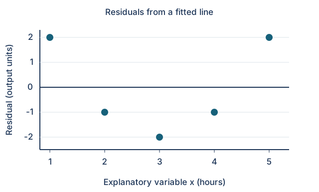
The residual plot below comes from fitting a least-squares line to five paired quantitative observations. The explanatory variable x is measured in hours and the residual is in output units. Each point is one observation.
Part a
What does the visible pattern suggest?
The U-shaped residual pattern is systematic curvature rather than random scatter about zero. It suggests that a straight-line model misses part of the association. A fitted least-squares line can have residuals that sum to zero even when the model form is inadequate; that property neither proves linearity nor establishes causation.
| Evidence for credit | Points |
|---|---|
| Select C. This item earns one point for the correct choice; the worked answer explains the reasoning. | 1 |
40. An intercept beyond the data: worked answer
A least-squares line predicts bus travel time y, in minutes, from route distance x, in kilometers: . The observed distances range from 3 to 15 kilometers.
Part a
Which interpretation of the intercept is most appropriate?
The intercept is the predicted response when x=0: 8 minutes. Because no route distance near 0 was observed, treating this as a reliable real route time requires extrapolation. The slope, 2.5, gives the predicted change per kilometer; the fitted intercept does not establish a universal physical waiting time.
| Evidence for credit | Points |
|---|---|
| Select B. This item earns one point for the correct choice; the worked answer explains the reasoning. | 1 |
41. Explained price variation: worked answer
For a sample of fruit boxes, a least-squares line predicts sale price y from box mass x. The correlation is r = 0.90, and a straight-line model is appropriate for the observed range.
Part a
Which calculation and interpretation of the coefficient of determination are correct?
Squaring the correlation gives r²=(0.90)²=0.81. The response is price, so r² describes the fraction of its observed variation explained by the linear relationship with mass. Reversing explanatory and response variables gives the wrong contextual interpretation, and explained variation is not an individual price fraction or a causal effect.
| Evidence for credit | Points |
|---|---|
| Select D. This item earns one point for the correct choice; the worked answer explains the reasoning. | 1 |
42. Fitting a least-squares line: worked answer
For five comparable shifts, x is the number of employees at a service counter and y is completed orders per minute. The paired observations are below. Use technology or a least-squares calculation to fit y on x.
| x (employees) | 1 | 2 | 3 | 4 | 5 |
|---|---|---|---|---|---|
| y (orders/minute) | 2 | 4 | 5 | 4 | 6 |
Part a
Which is the least-squares regression line?
The means are and . The least-squares slope is , and the intercept is . The line therefore predicts orders per minute as , and it passes through (3,4.2). Neither swapping coefficients nor drawing a line through selected points produces the least-squares fit.
| Evidence for credit | Points |
|---|---|
| Select A. This item earns one point for the correct choice; the worked answer explains the reasoning. | 1 |