One Mean and Paired Differences: A Complete t Investigation

These lessons and problems are newly written for the revised course. Worked examples show complete reasoning; the application questions ask you to make and defend your own choices.

Why estimating variability changes the distribution

A population mean μ describes the typical value of a quantitative response over a named population. Usually population standard deviation σ is unknown, so sample s estimates it. Treating s as a known population quantity would understate the uncertainty in a standardized mean. Student’s t distributions provide the reference family for critical values and test statistics in these mean procedures.

The t family is symmetric, bell-shaped and standardized, with heavier tails and a lower peak than the standard normal, especially at small degrees of freedom. Its df parameter depends on sample size; for one sample it is n−1. As df increases, the t curve approaches the standard normal, whose mean is 0 and SD is 1. This shape change explains why a small sample uses a larger 95% critical multiplier than z*=1.96. A sample SD is not a standard error: the latter describes the estimated variation of the sample mean over repeated samples.

One sample can be a sample of differences

For one sample of a quantitative response with unknown σ, estimate μ with a one-sample t-interval and test it with a one-sample t-test. Define the response, units and population: for example, mean perfume longevity in hours for a focus-group population. A statement such as “the average lasts longer” without a population or unit leaves the parameter unclear.

A matched-pairs design measures two dependent responses on the same person or on matched units. Form one difference for each pair in a stated order, then analyze the one sample of differences. The parameter μ_d is the population mean of those ordered differences. One-sample t methods apply to μ_d, with sample mean x̄_d as point estimate. n counts pairs, not twice as many individual measurements. Differences can be stable even when the original columns vary widely; their SD, not a pooled SD of those columns, belongs in SE.

For the ordinary mean, H₀:μ=μ₀; alternatives μ<μ₀, μ>μ₀ or μ≠μ₀ answer less, more or different questions. For after-minus-before change, H₀:μ_d=0; alternatives μ_d<0, μ_d>0 or μ_d≠0. If you reverse the subtraction, the sign and directional interpretation reverse too. Paired before/after observations without randomized control do not automatically establish that an intervention caused the change. Random treatment assignment and random population selection provide different support.

Check the distribution you actually analyze

Both one-sample t intervals and tests require randomization: a random sample or a randomized experiment. When sampling without replacement, verify n≤10%N using the population of sampled people/units; for paired population sampling, use the number of pairs. Population sampling is different from randomized treatment assignment, so there is no without-replacement population fraction to apply merely because an experiment assigns treatments.

The sample-data condition has alternatives: a stated approximately Normal population, or n≥30, or, for n<30, a sample distribution free of strong skewness and outliers. For paired data this must refer to the differences: at least 30 differences gives the large-sample route; with fewer than 30, inspect the sample of differences for strong skewness and outliers. Do not inspect only the before and after columns. A random design cannot fix a severe small-sample shape problem. The course’s large-sample threshold supports the approximation, but extreme measurements still deserve practical inspection rather than a blanket claim that large n makes every model reliable.

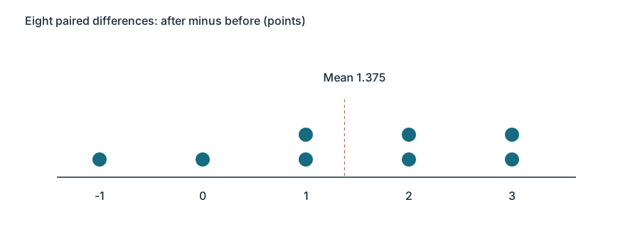
A new worked paired sample has eight after-minus-before changes: −1,0,1,1,2,2,3,3 points. Suppose an SRS of eight learners was selected from 2,000 learners. Randomization is given and 8≤200. The differences have no isolated extreme and a roughly balanced distribution; that supports the small-sample condition. Compare a sample −1,0,0,1,1,2,2,30: its isolated 30 undermines that condition even if its original columns happen to look harmless.

Compute the mean’s uncertainty and the t result

For the paired worked data, x̄_d=1.375 points, s_d≈1.407886 points, n=8. SE=s_d/√8≈0.497763 points. For an ordinary mean the same formulas use x̄ and s; x̄ or x̄_d is the appropriate point estimate. SE estimates variation of that mean across repeated samples, rather than the spread among individual differences.

Testing μ_d=0 against μ_d≠0 gives t=1.375/0.497763≈2.76236, df=7. Under the null, the statistic has a t₇ distribution; a table or technology gives the two-tail p≈0.0280006. For the central 95% t₇ area, t*=2.364624. The MOE is t*SE≈1.177022 points, so the confidence interval is (0.197978,2.552022) points.

For a separate one-mean worked sample, 16 generated perfume durations are 11.1,11.4,11.6,11.8,11.9,12.0,12.1,12.2,12.3,12.4,12.5,12.6,12.7,12.8,13.0,13.2 hours. Their mean is 12.225, s≈0.580230, SE≈0.145057. Against μ₀=12, t≈1.551109 with df15 and two-sided p≈0.141715. Using t*=2.131450 gives MOE≈0.309183 and 95% interval (11.915817,12.534183) hours. These newly supplied observations form a worked example; they do not complete missing historical stimuli or recover an unseen key.

Interpret probability, confidence and the investigative result

For the paired example, p≈0.0280 means: if the population mean after-minus-before change were zero, a sample of eight under this design would produce a standardized mean at least 2.76236 away from zero in absolute value with probability about 0.0280. Both tails are relevant to “change”; one upper tail is only half this two-sided probability. At α=0.05, p≤α gives reject H₀. There is convincing evidence of a population mean change among the sampled learner population, without proving a causal effect or claiming every learner improved.

We are 95% confident that the population mean after-minus-before change lies between 0.198 and 2.552 points. The endpoints are a lower and upper bound for the mean, not for individual changes. This entirely positive interval supports an increase in the population mean. The confidence level means that in repeated same-size samples from the same population, about 95% of intervals constructed this way contain the fixed μ_d. One computed interval either contains μ_d or does not; it is not correct to assign it a random population parameter.

For the separate perfume example, p≈0.1417>0.05 gives fail to reject μ=12. The interval includes 12, so it does not supply convincing two-sided evidence against that value. Neither result proves μ=12. A formal conclusion compares p with the preset α, names the parameter and population, follows the alternative, and uses limited evidence language. It is how the statistical result answers the original investigative question. A central 95% interval matches a two-sided 5% test; do not automatically reuse that match for a one-sided test.

Plan confidence and sample size together

For a fixed sample, increasing confidence requires a larger critical t*, which increases MOE and full interval width. At df24, 90% t*=1.710882 and 95% t*=2.063899. With n=25 and s=10 hours, SE=2; MOE rises from 3.421764 to 4.127798 hours, so the full width rises from 6.843528 to 8.255596 hours. Confidence buys a higher long-run capture rate by reporting a wider range.

Increasing n reduces SE when variability remains comparable. At fixed confidence, width is approximately proportional to 1/√n. Quadrupling n roughly halves the width; it does not quarter it. The relationship is approximate for t intervals because df and therefore t* also change. With n=100, s=10 and 95% t*=1.984217, SE=1 and width=3.968434, slightly less than half the n25 width. Decide which precision and confidence matter before choosing a sample-size target; higher confidence and smaller MOE cannot be obtained for free from the same data.

Independent Application

Work through each investigation before opening the separate solutions. State parameters, show calculations and connect your reasoning to the actual study.

Original generated practice for the Fall 2026 course.

A fully specified perfume investigation

This newly written problem retains the recorded perfume observations and supplies new complete instructions and independently computed answers. An SRS of 16 people is selected without replacement from a focus-group population of 4,000. Each tests the same perfume once; the response is hours of longevity. Population standard deviation is unknown. The question is whether the population mean differs from 12 hours; use α=0.05 and a 95% interval. Sorted data may be used to assess shape. For df=15, t*=2.1314495 and P(T≥2.6491522)=0.00911110.

Recorded perfume longevity observations (hours)

Observation	Hours
1	11.14
2	13.06
3	12.11
4	13.25
5	13.33
6	12.36
7	11.77
8	13.69
9	12.56
10	11.83
11	13.42
12	12.29
13	12.99
14	12.05
15	14.01
16	11.25

Part a

Define the population parameter in context and choose both the test and interval procedures. Explain why they use t rather than a standard normal critical value. State H₀ and Hₐ, then give the two alternative one-sided hypotheses for different questions about the same population.

Your reasoning

Part b

Justify all three conditions for both chosen procedures. Use a sorted dotplot, boxplot or explicit data summary to address skewness/outliers rather than saying that 16 is “large.”

Your reasoning

Part c

Calculate the point estimate, sample standard deviation, standard error, t-statistic, df and two-sided p-value. Interpret the p-value in context, explicitly naming the null assumption and both tails.

Your reasoning

Part d

Construct the 95% confidence interval, showing the margin of error and critical distribution/df. Interpret the interval and confidence level separately. Explain whether it supports the claim μ=12.

Your reasoning

Part e

Make the formal hypothesis-test decision and answer the longevity question with a qualified conclusion that names the parameter and population. Explain why the one shaded upper tail alone would not represent this two-sided p-value.

Your reasoning

Worked answer and rubric

Does instruction change the mean score?

An SRS of 12 learners is selected without replacement from 2,400 enrolled learners. Each takes a test before and after instruction. Scores are measured in points. Analyze the population mean change, defined as after minus before. Population variability of differences is unknown. This observational before/after design has no randomized control group; the question is evidence of a mean change, not proof that instruction alone caused it. Use α=0.05 and a 95% interval. For df=11, t*=2.2009852 and P(T≥7.4551289)=0.00000634549.

Same learners before and after instruction (test points)

Learner	Before	After
1	50	51
2	75	77
3	60	62
4	82	85
5	58	61
6	95	99
7	64	68
8	88	93
9	72	77
10	91	97
11	68	74
12	85	92

Part a

Form the twelve differences in the stated order, calculate their mean and sample SD, and identify the parameter. Select the interval and test methods. Explain why treating the two columns as independent samples would discard the design.

Your reasoning

Part b

State H₀ and the two-sided Hₐ for mean change; give the one-sided alternatives for increase and decrease. Justify randomization, sampling fraction and small-sample shape for the test and interval, using the differences rather than the separate columns.

Your reasoning

Part c

Calculate SE, t, df and the two-sided p-value. Interpret the p-value and decide whether the data provide convincing evidence of a mean change.

Your reasoning

Part d

Construct and interpret the 95% interval for μ_d, including its SE, MOE and critical df. Interpret its confidence level and use the interval to justify a claim about the direction of mean change.

Your reasoning

Worked answer and rubric

What distribution must look reasonable?

Each investigation concerns a one-sample mean or paired mean difference with unknown population σ. All sampling is without replacement. No device or participant appears twice except for the explicitly paired before/after measurement.

Design and shape information for four investigations

Study	Design	Size and distribution
A	SRS from 3,000 devices	8 lifetimes; population Normal
B	SRS from 3,000 devices	40 lifetimes; no population-shape information
C	SRS of paired participants from 3,000	40 after-minus-before differences
D	SRS of paired participants from 3,000	8 differences: −1,0,0,1,1,2,2,30

Part a

For each study, justify whether the randomization and 10% conditions are met and whether the course’s sample-data condition supports a one-sample t test/interval. Explain the population-Normal, n≥30 and small-n alternatives, and count pairs correctly.

Your reasoning

Part b

A fifth study randomly assigns two treatments within 10 matched pairs of volunteers. Its differences are −1,0,0,1,1,1,2,2,3,3, with no strong skew/outlier. Choose the t-method and explain randomization, which data need a shape check, and whether a sampling-without-replacement population bound is relevant to this experiment. Distinguish treatment inference from population generalization.

Your reasoning

Worked answer and rubric

Why the margin changes

A representative mean-lifetime study has n=36, sample s=12 hours, unknown population σ and approximately symmetric sample with no outliers. Central t critical values: df 35, 90%: 1.68957246; df 35, 95%: 2.03010793; df 143, 95%: 1.97669220. Standard normal central 95% critical is 1.959964. A second independently collected sample has n=144 and the same sample SD, confidence level and population. No mean is needed for width comparisons.

Part a

Describe the t family, its symmetry, tail/peak behavior for low df and its approach to the standard normal as df grows. Explain why this study uses sample s and t critical values rather than known σ and z. State the relevant normal limiting mean and SD.

Your reasoning

Part b

Calculate SE and MOE for 90% and 95% intervals at n=36. Explain the direction of critical value, MOE and full interval width when confidence increases for this fixed sample.

Your reasoning

Part c

Calculate the 95% SE, MOE and width at n=144. Compare to n=36 and explain the approximate 1/√n relationship, including why the exact ratio is not exactly one half here.

Your reasoning

Worked answer and rubric

Does a result prove the advertised mean?

A valid SRS investigation of battery life tests H₀:μ=36 hours against Hₐ:μ<36 hours for a model’s entire customer-use population, at prespecified α=0.05. Population σ is unknown. A correct one-sample t analysis produces a lower-tail p-value of 0.22. A separate 95% two-sided interval from these observations is (34.8,37.0) hours.

Part a

Interpret the p-value conditionally, make the formal decision and answer the investigative question with a limited population-mean conclusion. Explain why “μ=36 has been proven” is not supported.

Your reasoning

Part b

Interpret the interval and its endpoints and repeated-sampling confidence meaning. Use it to assess the advertised mean and the claim that every battery lasts between 34.8 and 37.0 hours. Explain why one should not automatically equate this two-sided interval with a one-sided 5% test.

Your reasoning

Worked answer and rubric