Two-Way Tables: Homogeneity and Independence

These lessons and problems are newly written for the revised course. Worked examples show complete reasoning; the application questions ask you to make and defend your own choices.

Let the sampling design name the test

A two-way table is a display, not a complete study design. If independent samples come from two or more populations and one categorical response is compared, a chi-square homogeneity test asks whether their response distributions are the same. Three independently sampled towns and one commute category fit this design. Identify the response variable and every target population when stating the question.

If one random sample from a single population records two categorical variables on each individual, a chi-square independence test asks whether those variables are associated in that population. One sample of city residents, each classified by dwelling and park-visit frequency, fits this design. State both variables and the population. Row labels alone do not tell us that two independent samples were selected. Quantitative averages, paired numerical changes and categorical counts call for different methods.

For homogeneity, H₀ says the categorical response distributions are the same across populations or randomized treatments; Hₐ says a difference exists. The alternative need not mean every pair differs. For independence, H₀ says no association, equivalently the variables are independent in the population. Hₐ says association, equivalently not independent. These claims concern distributions and variables, not whether every displayed count is equal.

Calculate what the null would expect

Under a shared distribution or independence, the expected count in a cell is its row total times column total divided by the whole-table total. Expected counts need not be integers. They are the null model’s predicted counts, not new observed people.

In a new worked example, independent SRSs of 60 people from each of three large towns give commute counts (walk,bus,drive): A=(30,20,10), B=(20,20,20), C=(10,20,30). Each row total is 60; each column total is 60; total 180. Thus every expected cell is 60(60)/180=20.

The randomization condition for independence is one random sample; for homogeneity it is independent random samples or a randomized experiment. For sampling without replacement, check n≤10%N in the relevant sampled population(s). The sampling condition is unnecessary when the data arise from randomized treatment assignment rather than population sampling. Random assignment and random selection support different scopes of conclusion. Finally, every expected count must be greater than 5. The required comparison is strict: an expected count exactly 5 does not meet it. Use expected rather than observed counts. In the worked town example, suppose each town has at least 3,000 people: 60≤300 and all expected counts 20>5, so all three conditions have concrete support.

Add discrepancies across the entire table

The chi-square statistic measures observed-versus-expected distance relative to expected counts. Squaring makes a deficit and an excess both contribute positively; division by E scales the contribution. Sum over all cells, including zero-contribution cells, rather than selecting the most dramatic row.

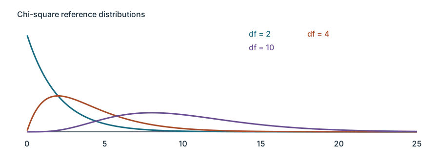
The worked table has four cells 10 away from their expected 20, each contributing 100/20=5, and five cells at their expected count, each contributing 0. Therefore χ²=20 and df=(3−1)(3−1)=4. Under H₀, the approximate reference distribution is chi-square with df=4; a table or distribution technology gives upper-tail p≈0.0004994.

Chi-square distributions have positive support and right skew; the statistic itself can be zero when every observed count equals its expectation. Increasing df makes the right skew less pronounced. Larger statistics mean more discrepancy, so p-values use the upper tail, regardless of whether particular cells have positive or negative O−E. Do not double this tail merely because some cells are above and others below expectation.

Answer the distribution or association question

The worked p-value means: assuming the three town commute distributions are the same, the probability of a table yielding a chi-square discrepancy at least 20 in these samples is about 0.0004994. It does not mean there is a 0.04994% chance the towns are the same. At α=0.05, p≤α gives reject H₀. There is convincing evidence that commute-choice distributions are not all the same across these town populations. The test is an omnibus comparison; it does not identify every differing category or establish that town residence caused the pattern.

For independence, interpret the probability assuming the two variables are independent in the sampled population. A small p supports an association; a larger p>α gives fail to reject and a statement that evidence of association is insufficient. It does not prove independence. State conclusions in context, consistently with the alternative and with non-definitive evidence language. The investigation concerns one sampled population for independence or several sampled populations for homogeneity; preserve that distinction when answering the original question.

Independent Application

Work through each investigation before opening the separate solutions. State parameters, show calculations and connect your reasoning to the actual study.

Original generated practice for the Fall 2026 course.

Are commute distributions the same across towns?

Independent SRSs of 90 working adults are drawn without replacement from each of three towns, each with at least 5,000 working adults. Each adult reports one primary commute choice: walk, bus or drive. Researchers ask whether the categorical commute distribution is the same in all towns, using α=0.05.

Observed commute choices in three towns

Town	Walk	Bus	Drive	Total
A	45	30	15	90
B	30	30	30	90
C	15	30	45	90
Total	90	90	90	270

For a chi-square distribution with 4 degrees of freedom, P(χ²≥30)=0.00000489444. This is an upper-tail probability, supplied so no particular calculator is required.

Part a

Choose the test and explain how the sampling design determines it. Identify the categorical variable and populations. State both hypotheses in context without implying that only two category percentages are compared.

Your reasoning

Part b

Find all expected counts, showing one row-total/column-total calculation. Then justify every required condition, including whether observed or expected counts determine the count condition.

Your reasoning

Part c

Calculate each distinct cell contribution and the whole chi-square statistic, the degrees of freedom and p-value. Describe the relevant distribution and why the tail is upper rather than lower or doubled.

Your reasoning

Part d

Interpret the p-value conditionally and decide at α=0.05. Answer the investigative question in context and explain what the test does not identify on its own.

Your reasoning

Worked answer and rubric

Are dwelling type and park visits associated?

An SRS of 200 residents is selected without replacement from a city of 25,000 residents. Each resident is classified by dwelling type and usual park-visit frequency. The question concerns association between these two categorical variables in this city population, using α=0.01.

Observed park visit by dwelling type

Dwelling	Daily	Weekly	Less often	Total
Apartment	50	30	20	100
House	30	40	30	100
Total	80	70	50	200

A chi-square upper-tail calculation gives P(χ²₂≥8.428571)=0.01478288.

Part a

Select the test and explain why this design differs from independent samples from several populations. State H₀ and Hₐ in both association language and independence language, identifying the population and both variables.

Your reasoning

Part b

Calculate all six expected counts and justify the three conditions. Compute each contribution to χ², its sum and df. Use the supplied tail probability to find the p-value.

Your reasoning

Part c

Interpret the p-value and conclude at α=0.01. A resident says “The test establishes independence.” Explain why this statement is too strong and compare the decision if α had been 0.05.

Your reasoning

Worked answer and rubric

What makes a chi-square analysis defensible?

Study A randomly assigns 120 volunteers, 40 to each of three snack packages, and records one of three preference ratings. Every null expected cell is 12 or more. Study B is one SRS of 80 households without replacement from a population of 400; each household is classified by dwelling tenure (own/rent) and heating type (gas/electric/other); its smallest expected cell is 9. Study C uses independent SRSs from two towns, records primary commute category (walk/bus/drive) and each sample no more than 5% of its population, but one expected cell is exactly 5. Study D measures numeric travel times and compares averages. The investigators want to compare population/treatment response distributions or association as their designs allow.

Part a

For A–D choose homogeneity, independence, a mean procedure, or explain why the proposed chi-square approximation is not justified. For A–C explicitly discuss randomization, the 10% condition and the strict expected-count requirement. Explain the scope of A’s conclusion.

Your reasoning

Part b

Describe how χ² measures discrepancy and how the shape changes between df=2 and df=10. Explain why a negative test statistic or a lower-tail p-value would signal a calculation/interpretation error.

Your reasoning

Worked answer and rubric