Reading SHM: Worked Solutions

Try the questions on the lesson page first. Then compare both the answer and the reasoning. The worked steps here are original.

Question 1: At the positive turning point of ideal SHM, which pair is correct?

At the positive turning point of ideal SHM, which pair is correct?

1. At the positive turning point, x = +A. Why: The cart has reached its greatest positive displacement.
2. Read the horizontal tangent of x(t): v = 0. Why: Velocity is the slope of the position graph.
3. Use a = −ω²x: acceleration is most negative. Why: The greatest positive displacement creates the greatest leftward restoring acceleration.

Try this question again.

Question 2: Amplitude doubles while m and k stay fixed. What changes?

Amplitude doubles while m and k stay fixed. What changes?

1. Keep m and k fixed, so ω = √(k/m) is unchanged. Why: These variables set the ideal frequency and period.
2. Use v_max = Aω to compare amplitudes. Why: Maximum speed is directly proportional to A at fixed ω.
3. Doubling A doubles maximum speed and leaves period fixed. Why: The graph stretches vertically while the time between repeated states stays the same.

Try this question again.

Question 3: Position crosses its equilibrium midline with a negative slope. The cart is…

Position crosses its equilibrium midline with a negative slope. The cart is…

1. Read a negative slope of position versus time as negative velocity. Why: The slope shows the direction of travel, so the cart is moving left.
2. At the midline, displacement from equilibrium is zero. Why: The sensor midline represents the coordinate used in the restoring equation.
3. Use a = −ω²x to get a = 0. Why: Zero acceleration at that instant does not imply zero velocity.

Try this question again.

Question 4: a graph and a symbolic comparison

A position graph has peaks +0.050 m and troughs −0.050 m, with successive positive peaks 0.40 s apart. Find its maximum speed. A second oscillator has the same amplitude and half the period. Compare their maximum accelerations.

1. Read A = 0.050 m and T = 0.40 s, giving ω = 2π/T. Why: Amplitude is the distance from midline to a peak, not the full peak-to-peak distance.
2. Calculate v_max = Aω = 2π(0.050)/0.40 = 0.785 m/s. Why: The steepest position slope gives maximum speed at equilibrium.
3. Use a_max = 4π²A/T²: halving T multiplies a_max by 4, from 12.3 to 49.3 m/s². Why: The frequency factor is squared in acceleration. A second position curve has equally high peaks but peaks twice as close in time.

Try this written problem again.

Question 5: turn measured positions into a graph

A motion sensor records displacement from equilibrium for a horizontal spring cart. Its position uncertainty is approximately ±0.002 m; assume negligible friction and an ideal linear spring. Plot the measured positions below on a numerical x-versus-t graph with labeled units and scales, then sketch a smooth trend. Estimate amplitude and period from the graph and calculate maximum speed. On aligned qualitative velocity and acceleration graphs, mark the signs and important features at t = 0.20 s and t = 0.40 s. Explain whether the measured points are consistent with an SHM model, while recognizing what a short data record can establish.

Time t (s)	Measured displacement x (m)
0.00	+0.081
0.10	+0.056
0.20	+0.001
0.30	−0.057
0.40	−0.079
0.50	−0.056
0.60	−0.001
0.70	+0.057
0.80	+0.080

View the worked graph at full size ↗

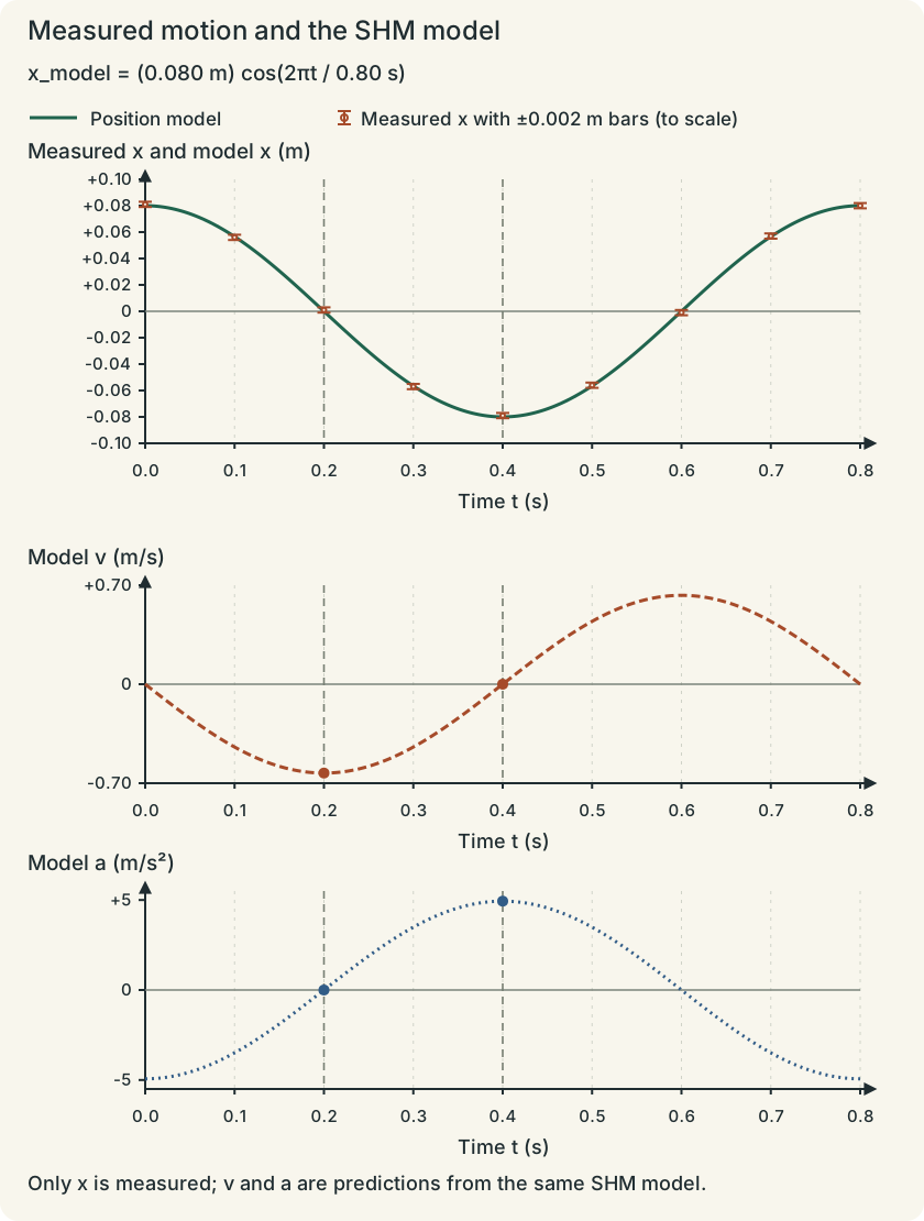
1. Use a horizontal time axis from 0.00 to 0.80 s, such as ticks every 0.10 s, and a vertical displacement axis from −0.10 to +0.10 m, such as ticks every 0.02 m. Plot all nine measured points and draw a smooth sinusoidal trend near them. Why: A numerical plot needs usable scales and units. The measurements have uncertainty, so the physical trend need not pass exactly through every point.
2. Estimate A ≈ [0.081 − (−0.079)]/2 = 0.080 m. The successive positive peaks near 0.00 and 0.80 s give T ≈ 0.80 s and f ≈ 1.25 Hz. Why: Amplitude is half the peak-to-peak displacement. A period compares repeated positions with the same direction of subsequent motion, not adjacent opposite turning points.
3. Calculate ω = 2π/T ≈ 7.85 rad/s and v_max = Aω ≈ 0.628 m/s. Why: The greatest slope of the ideal sinusoidal position curve occurs at equilibrium and equals its maximum speed.
4. At about 0.20 s the curve crosses equilibrium moving left: velocity is most negative and acceleration is approximately zero. At about 0.40 s it reaches the negative turning point: velocity is zero and acceleration is most positive, about +4.93 m/s². Why: Velocity follows position slope, while a = −ω²x gives the restoring acceleration. The displacement minimum has a horizontal tangent but does not have zero acceleration.
5. An ideal trend x_model = (0.080 m)cos(2πt/0.80 s) differs from the listed positions by at most about 0.001 m, within the stated ±0.002 m uncertainty. The record is consistent with SHM but does not by itself prove the model uniquely; more cycles and a force-displacement test would add evidence. Why: Model checking compares predicted features with measurement uncertainty. Finite noisy measurements support a model without establishing every possible future behavior.

Try this written problem again.