Newton’s Second Law
Connect the external force sum to center-of-mass acceleration.
The net force changes the motion
Let’s push an empty shopping cart, then push the loaded cart with the same force. The loaded cart’s velocity changes more slowly. Push either cart harder and its velocity changes faster. Newton’s second law gives us the mathematical relationship behind that observation.
For a fixed-mass system in an inertial frame, ΣF⃗_external = M a⃗_CM. The acceleration of the system’s center of mass points in the direction of the net external force. Its magnitude is proportional to net force and inversely proportional to total mass. An unbalanced force configuration means the vector sum isn’t zero.
The direction of acceleration isn’t necessarily the direction of velocity. A cart can move right while the net force points left. It slows down at first, but may later reverse and speed up left if that force continues. Force predicts a change in velocity, not the current velocity itself.
Write the force sum, not just one force
For one axis, ΣFₓ = Ma_CM,x. Include all external components with signs. A 12 N pull right opposed by 4 N friction left gives net force +8 N, not +12 N. Balanced vertical forces don’t belong in the horizontal equation, but they still need their own force balance.
For a system of two connected carts, the forces they exert on each other are internal and cancel from the system sum. They still matter if you analyze one cart alone. Choosing the larger system often finds the common acceleration efficiently; choosing one part afterward can find the connecting tension.
Example 2.5.1 — A pair of carts
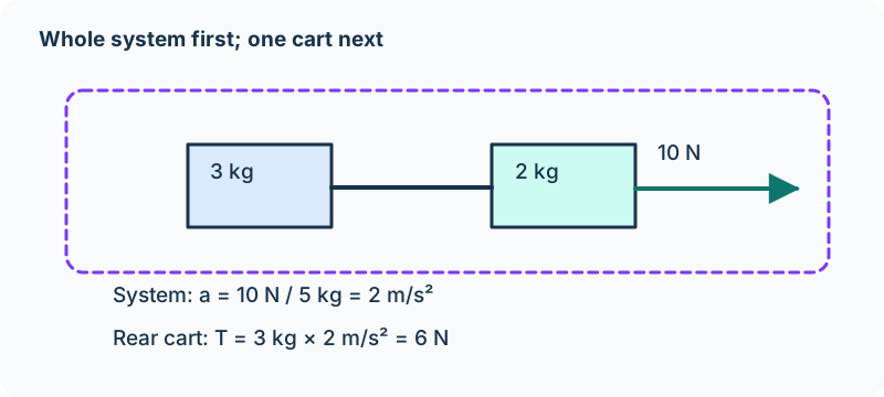
A 2 kg cart pulls a 3 kg cart along a frictionless horizontal track. An external 10 N force acts right on the 2 kg cart. The taut, ideal string keeps their acceleration magnitudes equal. For both carts together, total mass is 5 kg and net horizontal external force is 10 N. Thus a = 10/5 = 2.0 m/s² right.
For the 3 kg cart alone, the string supplies its only horizontal force: T = 3a = 6 N. For the 2 kg cart, 10 − T = 2a, and 10 − 6 = 4 N agrees with 2(2) = 4 N. The same T appears because the string is ideal; it doesn’t mean tension is external to the combined system.
Now add 2 N of opposing friction to each cart. The whole-system net force becomes 10 − 2 − 2 = 6 N, so acceleration is 6/5 = 1.2 m/s². For the rear 3 kg cart, T − 2 = 3(1.2), giving T = 5.6 N. Recalculate the force sum when the environment changes; don’t keep the previous tension by habit.
Use symbols to predict changes
If net force doubles with total mass fixed, acceleration doubles. If total mass triples with net force fixed, acceleration becomes one third as large. If both force and mass double, acceleration is unchanged. These claims hold only when the net force is actually held at the stated value.
Pulling a larger mass with the same hanging weight doesn’t automatically keep force on the cart constant: the hanging weight itself accelerates, so string tension can change. That is a reason to model both masses, or measure tension with a sensor rather than equating it to the hanging weight.
A graph can reveal the law
Use a force sensor and motion sensor on a low-friction cart. For several nearly constant pulls, measure net horizontal force and acceleration over the same time interval. Plot a versus F_net at fixed mass. The best-fit slope should be 1/M, with units kg⁻¹, and the intercept should be near zero if residual forces have been included.
Repeat with different total masses and a comparable measured net force, then plot a versus 1/M. Keep track slope, wheel behavior, and force-sensor calibration consistent. Repeated trials reduce random scatter; correcting a track tilt addresses a systematic effect. A meaningful procedure distinguishes those two kinds of improvement and explains what a slope tells you about the model.
A sliding incline block coupled to a hanging block
Assume a taut, negligible-mass, nonstretching rope and an ideal fixed pulley. Equal tension follows from these ideal assumptions, rather than from the system accelerating. The rope gives equal acceleration magnitudes along the two paths; the spatial acceleration vectors differ. While B slides downhill, friction acts uphill. Its uphill acceleration means it slows, not that it is already moving uphill; reconsider the friction regime when sliding stops.
Historical force/component construction diagrams. Gallery-6 combines gravity and projections; do not count projections as extra forces or present it as an AP exam FBD. Reference native dot-origin individual-force FBD instruction. Individual-force diagram conventions →
Notation and model qualifications in the retained source
- Equal tension follows from the ideal rope/pulley, not from acceleration. Original wording →
- The stray 40° attached to Block A belongs to Block B’s incline. Original wording →
Review the model and equations used here →
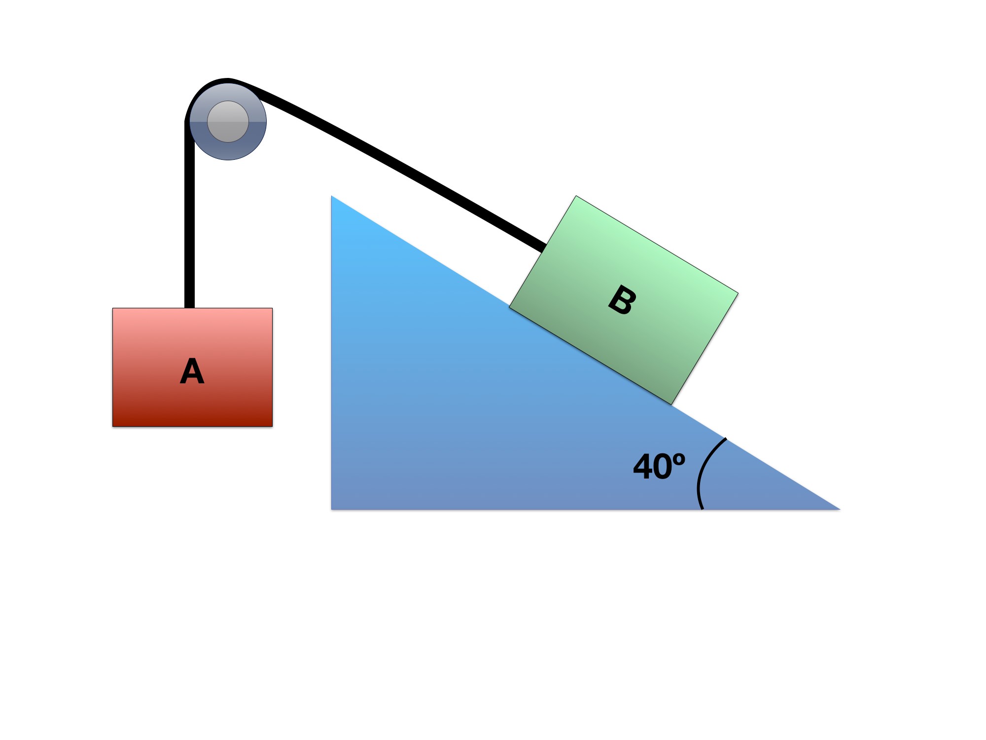
Blocks A and B, connected by a frictionless pulley.
A 4 kg hanging block A is connected over an ideal fixed pulley to an 8 kg block B on a 40° incline. Block B is currently sliding down the incline. Use μₖ = 0.3 and g = 9.81 m/s². Find each block’s acceleration and its direction.
The negative acceleration means block B accelerates uphill while block A accelerates downward. If B is currently sliding downhill, it slows; negative acceleration alone does not mean it is already moving uphill.
Block B’s acceleration is 0.569 m/s² uphill; block A’s acceleration is 0.569 m/s² downward.
Therefore:
The EOM for block B in the x direction is:
so:
and in the y- direction there is no acceleration so sum of forces in y-direction for block B is zero! Thus, we can set the normal force and the y component of the gravity force equal to each other.
Step 1: Set up your Free Body Diagram
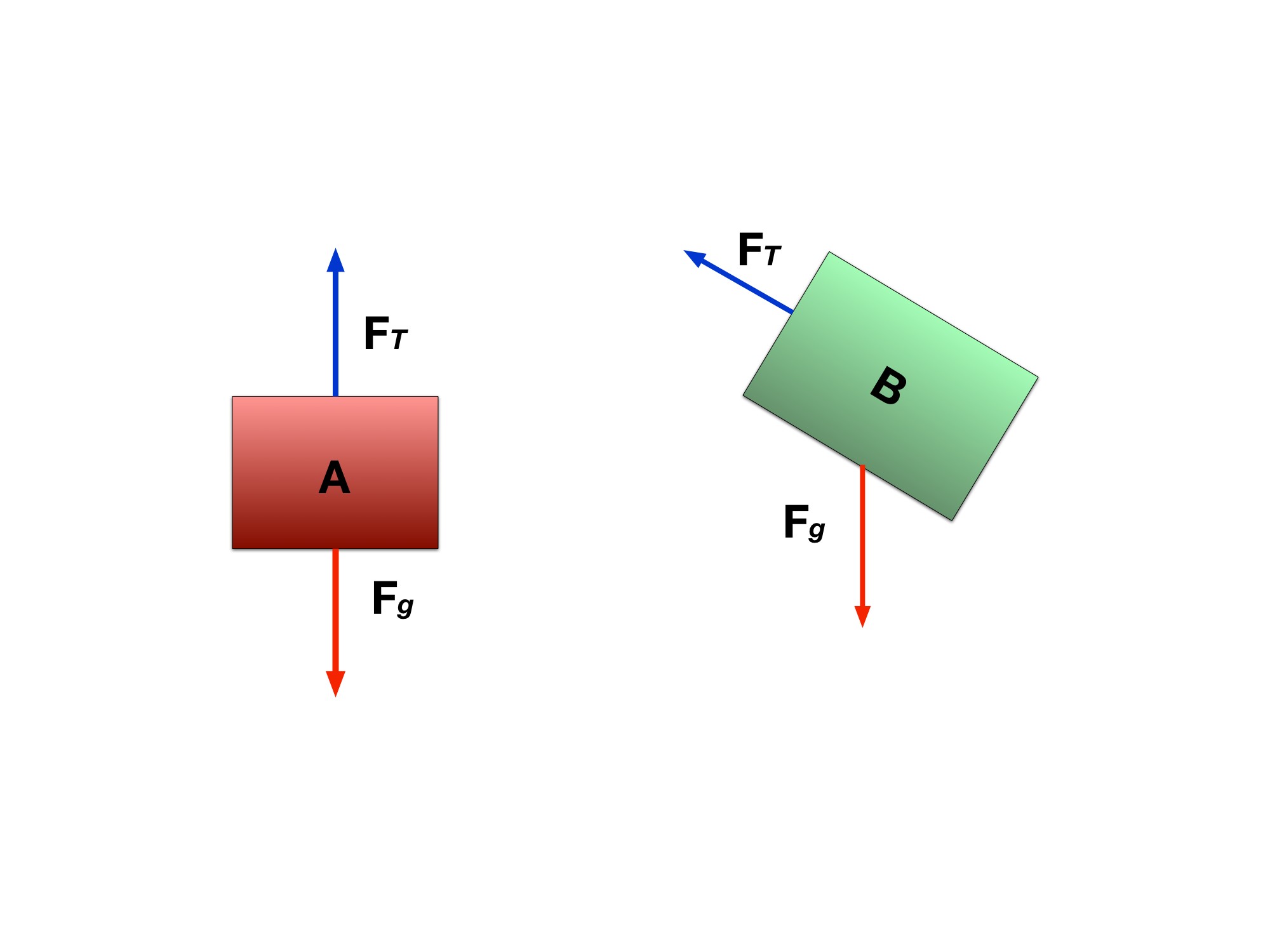
Reference the image in this Gallery to view the FBD. Notice here that there are two FBDs constructed and two reference axes, one for block A, the other for block B. Each of the reference frames are oriented in the same direction as the object. Remember that we can set our reference axes to whatever orientation we want. It’ll cause less of a headache for us when we’re setting up our equations of motion.
Step 2: Break up the forces into x and y components
Based off the FBD, let’s approach the forces that are on each block. The force breakdown can be seen in this here Gallery. For block A, we see that forces are only in the y-direction which are tension and the weight of block A.
According to the reference axes for block A, the weight is acting in the negative y-direction so:
For block A, T − m_Ag = m_Aa, with upward positive. For the currently downhill-sliding block B, the shared signed acceleration is a = −0.56915 m/s².
Notice how the acceleration is negative. Due to our reference axes, we are assuming that a positive movement would be block B moving down the plane and pulling block A up.
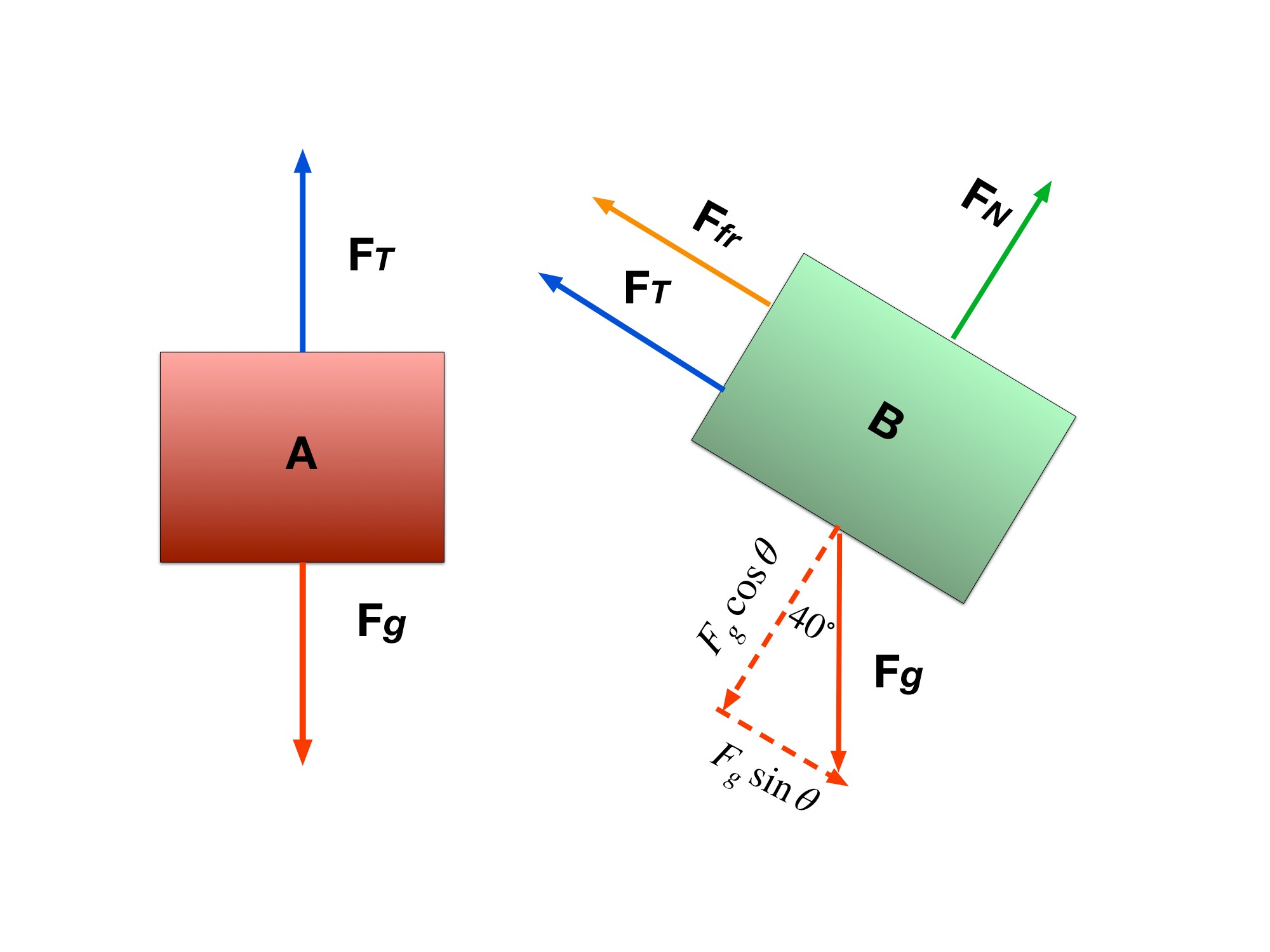
Here are the more detailed FBDs for each block. Friction, the normal force, and the gravity components are added.
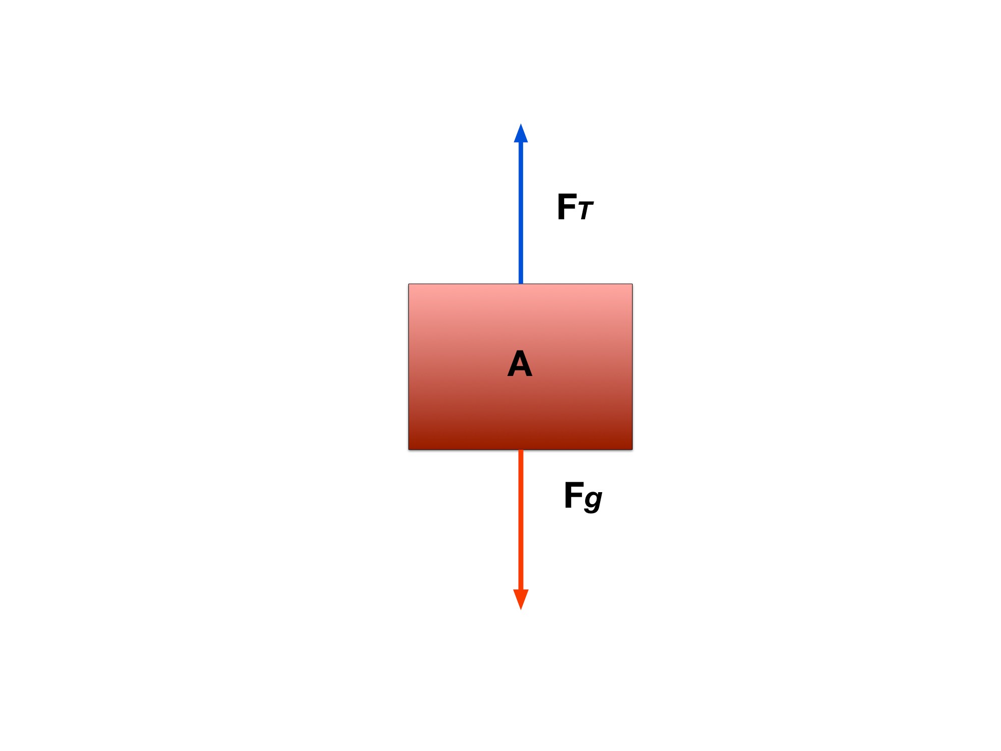
y-components for block A.
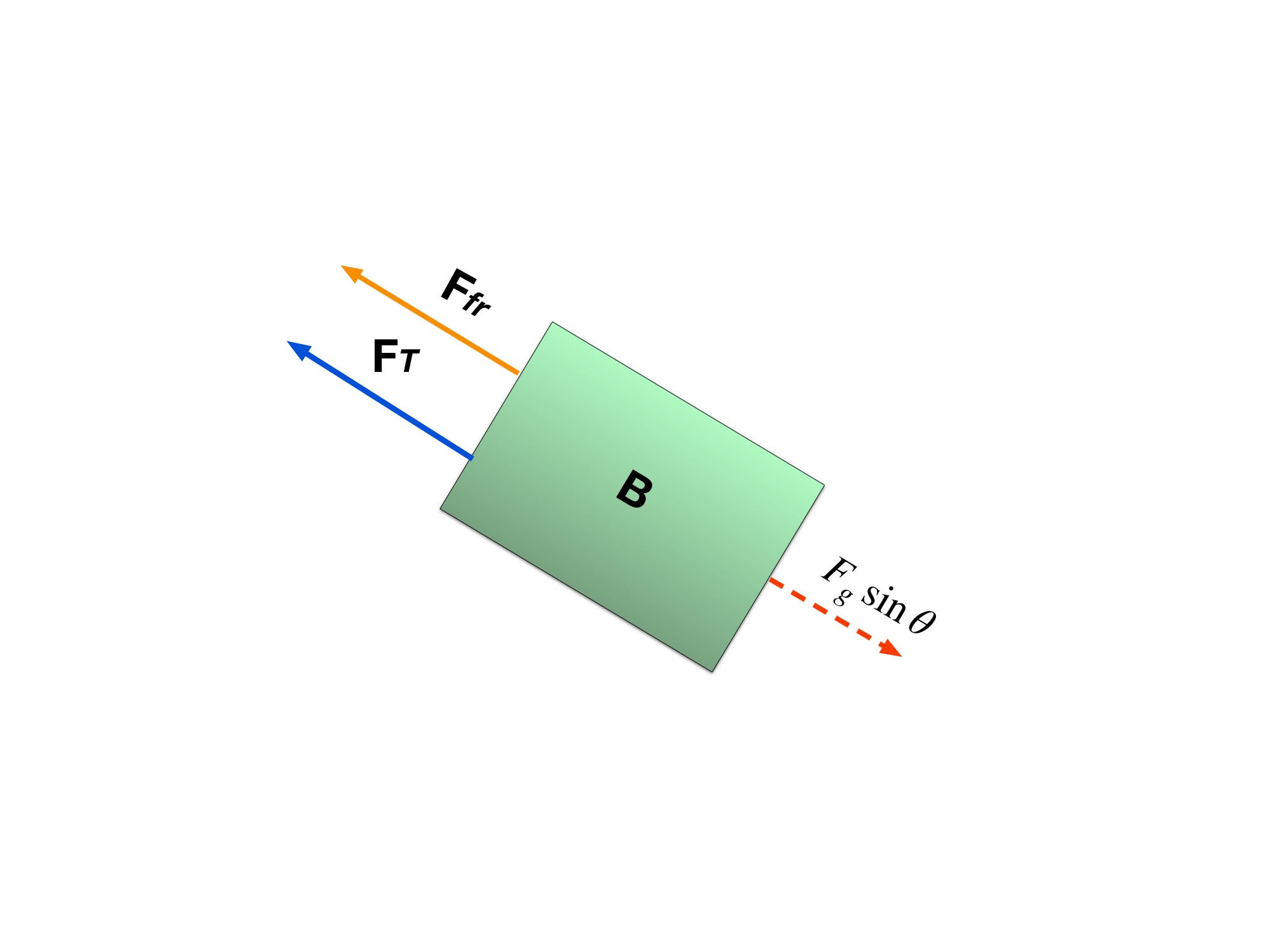
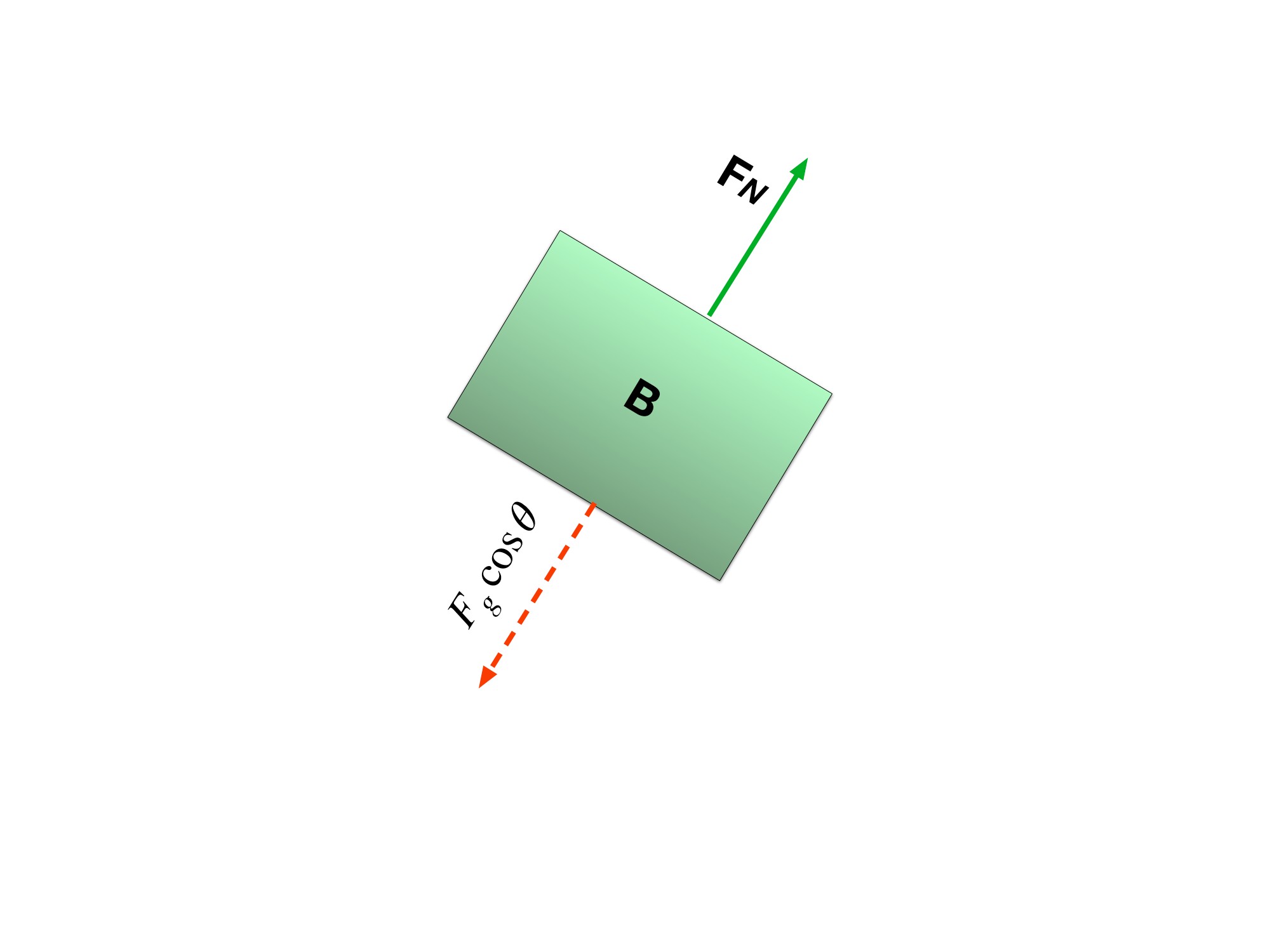
Notice how the Tension force is represented by just T for both blocks A and B. This is because we are concerned with how the system as a whole is accelerating so the tension force that is present in block A is the same as the tension force felt in block B. so we can rewrite the x-component of the force balance as:
and combine all the equations to get:
Step 4: Solve for the acceleration of the system
The rope constrains the two blocks to have equal acceleration magnitudes along their respective paths. Their acceleration vectors point in different spatial directions.
Physics I by Jake Yap and Laurence Vincent. Complete historical context and correction history →
Check what you know
Pause & try it
Let's see what stuck.
Choose an answer, then check the reasoning. Try the written problems below before opening their solutions.
0 of 3 checked · 0 correct
Give it a try
Practice 1
A 4 kg cart has a 15 N rightward pull and 3 N leftward friction. Find acceleration and the velocity change after 2 s of constant force.
Practice 2
For the two-cart example, derive a = F/(m₁ + m₂) and T = m₂F/(m₁ + m₂) on a frictionless track. Explain which system gives each equation.
Practice 3
A best-fit graph of a versus F_net has slope 0.25 kg⁻¹. Infer the mass. Explain how an unaccounted constant friction force would affect the graph’s intercept.
Keep exploring
The original Force Analysis and Common Forces preserve the connected-block problems. Analyze each with a stated system and external force sum.
Course scope and standards: the supplied AP Physics 1 CED, printed pages 49; Topic 2.5 and its exact learning objectives. The official College Board CED is the public source; the project audit records the supplied edition.
Supporting physics references: OpenStax: Newton’s second law and systems. These lessons, diagrams, examples, and practice questions were written for this book.
Related source reading
These alternative explanations and examples retain their source context. Draft placement does not add accepted exam coverage.
- Quadratic drag and terminal-speed balance · source context; placement review pending
Glossary and deeper reading · 11 refreshers
These editorial refreshers supplement the reading. Definitions and examples are added guidance; original source wording and recorded answers remain in their original context.
-
Force
A force describes an interaction that can change an object’s momentum. It is a vector measured in newtons, so both size and direction matter when forces are added. For example, a rope can pull a cart while the floor exerts friction in another direction.
-
Velocity
Velocity describes how position changes with time and includes direction. Instantaneous velocity describes one moment, while average velocity is displacement divided by elapsed time. For example, a car turning a corner can change velocity while maintaining the same speed.
-
Inertial frame
An inertial frame is a reference frame in which an object with no net external force moves at constant velocity. Frames moving at constant velocity relative to an inertial frame are also inertial in the Newtonian model. For example, a steadily moving train is approximately inertial, whereas a train accelerating out of a station is not.
-
Acceleration
Acceleration is the vector rate of change of velocity with time. It can change an object’s speed, direction, or both, and it is measured in meters per second squared. For example, a satellite moving at constant speed in a circular orbit accelerates toward the center.
-
Vector component
A vector component describes the part of a vector along a chosen axis. Its signed value changes when the axes change, even though the physical vector remains the same. For example, a diagonal launch velocity can be resolved into horizontal and vertical components that share the same elapsed time.
-
Tension
Tension is a pulling force transmitted through a stretched rope, string, or similar connector. It acts along the connector away from the object it pulls, and an ideal massless rope has the same tension throughout an uninterrupted segment. For example, a rope supporting an accelerating load can have a tension different from the load’s weight.
-
Weight
Weight is the gravitational force exerted on an object by a specified attracting body. Near Earth’s surface its magnitude is approximately mass times the local gravitational field strength, and it is measured in newtons. For example, an astronaut has less weight on the Moon while retaining the same mass.
-
Magnitude
Magnitude is the nonnegative size of a vector quantity. It does not specify direction, and it differs from a signed component. For example, a westward velocity can have a negative x component while its speed, the velocity magnitude, stays positive.
-
Vector
A vector is a quantity with a magnitude and a direction, represented by an arrow or by components along chosen axes. Vectors add by adding corresponding components rather than simply adding their magnitudes. For example, an eastward displacement followed by a northward displacement produces a resultant pointing northeast. The zero vector has zero magnitude and no unique direction.
-
Gravity
Gravity is the attractive interaction between masses in the Newtonian model. For spherical bodies or point-mass approximations, its strength decreases with the square of the separation between their centers. For example, Earth’s gravity provides the inward force that keeps a satellite in orbit.
-
Free-body diagram
A free-body diagram shows the external forces acting on one selected object or system. Each arrow names a real interaction, and its direction is the direction of that force. For example, a book resting on a desk has a downward gravitational force and an upward normal force; velocity is not an extra force arrow.