Correlation: Linear Strength, Direction, and Limits

An upward or downward pattern is easier to compare across settings when it has a numerical summary. The correlation coefficient describes a particular kind of pattern: linear association between two quantitative variables. Its strength is its usefulness and also its limitation.

What Correlation Measures

The correlation coefficient, written $r$, summarizes the strength and direction of a linear association. It is unit-free and always lies between −1 and 1, inclusive. A positive r indicates positive association; a negative r indicates negative association. The closer r is to either endpoint, the stronger the linear association. A value near zero indicates weak linear association.

Exactly $r=0$ means no linear association; it does not rule out a curved relationship. Exactly $r=1$ or $r=-1$ means a perfect positive or negative linear association: all plotted observations follow a non-horizontal straight-line relationship, assuming both variables vary. There is no valid correlation value of 1.2 or −1.4. The sign gives direction, while the distance from zero gives linear strength. A negative r is not automatically weaker than a positive r.

Correlation	Interpretation of linear association
−0.92	Strong negative
−0.20	Weak negative
0	None, although a non-linear pattern may exist
0.92	Strong positive
1 or −1	Perfect linear association

These strength words are descriptions rather than universal cutoff rules. Report context and inspect the plot as well. Because r has no units, measuring the same distances in centimeters rather than meters leaves r unchanged under that positive unit conversion. In contrast, a regression slope can change because its units change. A steep line can have the same correlation as a shallow line.

Worked Comparison

Two groups relate practice hours to target scores. Group A has r=−0.88; group B has r=0.63. Group A has the stronger linear association because 0.88 is closer to 1 than 0.63 is. Its direction is negative, while group B’s is positive. Saying that 0.63 is “larger” does not answer which relationship is stronger.

Check the Form Before the Number

A correlation close to −1 or 1 does not necessarily make a linear model appropriate. A curve can have a high correlation because its overall movement is consistently upward or downward, yet its shape systematically departs from a line. A small correlation also does not mean “the variables have no relationship.”

Worked Example: A High Correlation on a Curve

For the generated pairs (1,1),(2,4),(3,9),(4,16), technology gives $r\approx0.9844$. The association is positive and its linear correlation is high, but the plotted shape bends upward. The points follow y=x squared exactly. A curved model can describe that shape more faithfully than a straight line. The decision to use a linear model requires the scatterplot’s form, not just a favorable r.

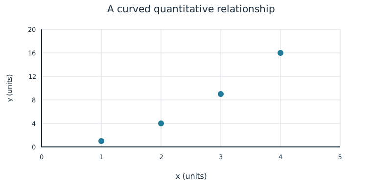
There can also be a strong U-shaped pattern with r=0. For example, the pairs (−2,4),(−1,1),(0,0),(1,1),(2,4) have no linear association because the two arms balance; they still follow a precise curve. Keep “linear” in any interpretation of zero correlation.

Association and Cause

A perceived or real relationship does not mean that changing one variable causes the other to change. Correlation does not necessarily imply causation. A third variable may influence both, individuals may select their own conditions, or the observed group may differ in other ways. The coefficient itself does not tell how the data were collected.

Suppose on warmer days a park sells more ice cream and rents more bicycles. A positive correlation between ice cream sales and bicycle rentals would not show that buying an ice cream causes a bicycle rental. Temperature and visitor numbers offer alternative explanations. In another study, random assignment of a treatment may support a causal conclusion when the design is appropriate; that conclusion comes from the study design, not from r alone.

Worked Claim

An observational sample finds r=0.81 between weekly practice hours and target score. It supports a positive linear association in that sample, subject to the scatterplot’s form and any unusual observations. It does not prove that assigning an additional hour of practice will cause any particular member’s score to rise. Prior experience could affect both chosen practice time and score. Interpret the evidence actually collected rather than a different experiment that did not occur.

Independent Practice

Use the information in each question to make your own calculation, representation, or argument. Explain what your result means in its setting.

Original generated practice for the Fall 2026 course.

Compare signs and strengths

An analyst reports r=−0.91 for distance from a lamp versus light reading, and r=0.54 for practice time versus target score.

Part a

Interpret both correlations in context and determine which has the stronger linear association. Explain your comparison.

Your reasoning

Worked answer and rubric

A coefficient cannot have meters

The same varying distance and light-reading observations are analyzed first with distance in meters and then in centimeters. The first output is r=−0.72. A second report prints r=−1.08 meters.

Part a

State the correlation after the positive unit conversion and explain why “−1.08 meters” cannot be a valid correlation. Include the allowed range and its endpoint convention.

Your reasoning

Worked answer and rubric

Zero and perfect correlations

For 80 measured library visits, both the number of books borrowed and visit duration in minutes vary. A complete calculation reports exactly r=0 for those two quantitative variables; no scatterplot is supplied. Separately, generated data set L contains (1,9),(2,7),(3,5),(4,3), with r=−1. Both variables vary in L.

Part a

Interpret r=0 for the library visits and r=−1 for L. Does the zero report establish that books borrowed and visit duration have no relationship of any form? Explain what remains possible when no plot is supplied. What would r=1 mean for a data set with both variables varying?

Your reasoning

Worked answer and rubric

An impressive number on a curve

The generated pairs are (1,1),(2,4),(3,9),(4,16). Their correlation is r≈0.9844.

Part a

A student says, “r is so close to 1 that a linear model must be appropriate.” Evaluate the reasoning using the scatterplot.

Your reasoning

Worked answer and rubric

Warm days at the park

Across 40 observed park days, ice cream sales and bicycle rentals have r=0.87. Neither quantity was assigned by researchers; warmer and busier days tend to have more of both.

Part a

Does the result establish that increasing ice cream sales causes more bicycle rentals? Interpret what r supports and give a context-specific alternative explanation.

Your reasoning

Worked answer and rubric

Review three quantitative reports

Three generated reports analyze varying numerical variables. Report A: weekly practice hours and target scores, r=0.82, with a roughly straight upward scatterplot and noticeable scatter. Report B: distance from a lamp and light reading, r=−0.96, with a roughly straight downward pattern. Report C: x and y with full pairs (1,1),(2,4),(3,9),(4,16), r≈0.9844. Practice hours in A were chosen by members, not assigned.

Part a

Interpret the sign and linear strength of A and B, compare their linear strengths, and state whether changing A’s hours to minutes would give r units or change its value.

Your reasoning

Part b

Report C has the largest positive r. Explain why that fact does not establish that its straight-line model is the best form.

Your reasoning

Part c

A club advertises, “Our correlation proves that forcing members to practice longer causes higher target scores.” Evaluate that statement and name one plausible common cause in this setting.

Your reasoning

Worked answer and rubric

Evaluate a coating-station report

A workshop records tray opening width and dispensed coating volume in five generated production trials. The width is used to explain the volume. All five observations are supplied below; the calculated correlation is r≈0.9845.

Complete measurements from five generated production trials

Trial	Tray opening width (cm)	Coating volume (mL)
1	2	6
2	3	13
3	5	29
4	7	56
5	9	91

Part a

Describe the scatterplot’s form, direction, strength and unusual features in this setting. Cite numerical changes or point positions that justify your description. Do not decide the form from r alone.

Your reasoning

Part b

An analyst says, “Because 0.9845 is nearly 1, we can choose a straight-line model without inspecting the plot.” Evaluate that claim. Explain both what this near-endpoint r measures and why it does or does not settle the model-form choice.

Your reasoning

Worked answer and rubric