Compare Quantitative Distributions and Relative Position
Two samples can differ in several ways at once. A clear comparison uses the same variable and units, considers both distributions explicitly, and separates typical position from spread or unusual extremes. A standardized score adds another kind of comparison: how far an individual value stands from its distribution’s mean.
Compare Ordered Graphs
Histograms, back-to-back stem-and-leaf plots, and dotplots can compare center, variability, shape, outliers, clusters, and gaps for two or more distributions of the same quantitative variable. Use comparable scales and the same bin rules. For different sample sizes, relative-frequency histograms can compare shares more clearly than raw counts.
Office A’s sampled commutes are 10,11,12,13,14,15,16,17 minutes. Office B’s are 8,10,12,14,16,18,20,34 minutes. A is fairly balanced around 13.5 minutes, with a compact range. B spreads farther, especially toward 34 minutes, and has a long upper tail and a gap above 20. In dots, A has one observation at each listed minute while B’s exact values show the long gap. Wider histogram bins merge this detail, so do not invent peaks or gaps that the chosen binning cannot show.
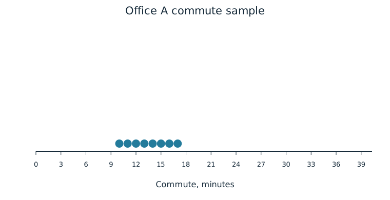
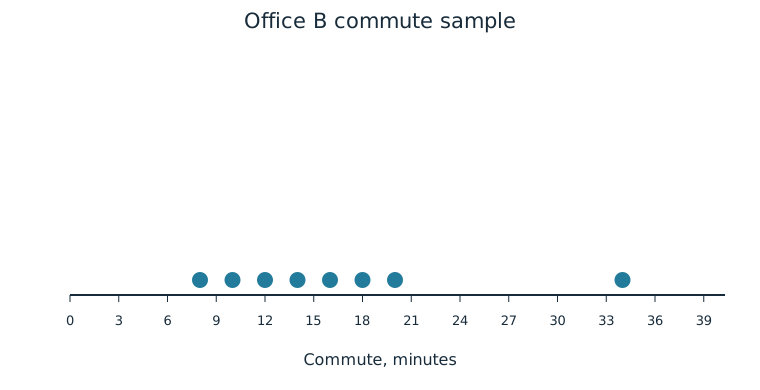
A back-to-back stem-and-leaf version gives an exact-value comparison on one set of stems:
| A leaves, read outward from stem | Tens stem | B leaves |
|---|---|---|
| 0 | 8 | |
| 7 6 5 4 3 2 1 0 | 1 | 0 2 4 6 8 |
| 2 | 0 | |
| 3 | 4 |
Key: left leaf 7 with stem 1 means 17 minutes; stem 1 with right leaf 0 means 10 minutes. No value is omitted when the stem has leaves on only one side.
Compare Summary Representations
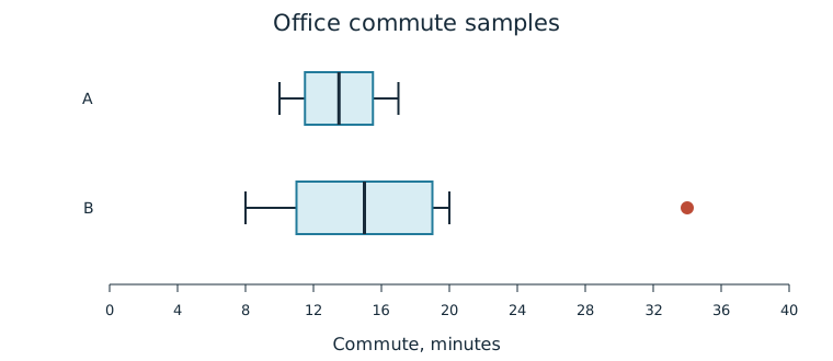
Boxplots can compare center, variability, outliers, and skewness or symmetry. They do not expose all internal clusters or gaps. Numerical summaries can supplement the graphs: A has mean/median 13.5 minutes, IQR 4 minutes, and SD about 2.449 minutes; B has mean 16.5, median 15, IQR 8, and SD about 8.124 minutes. B’s median is only 1.5 minutes above A’s, while its IQR is twice as large and its high outlier has a large effect on the mean and SD.
Justify a Comparison
To support “Office B’s commutes are more variable,” state the measure and evidence: IQR 8 versus 4, SD 8.124 versus 2.449, or observed range 26 versus 7 minutes. To assess “every B commute is longer,” note B’s 8-minute observation below every A value. Multiple quantitative graphical representations can support contextual claims, but the claims must fit the sample and cannot establish the cause of an office difference.
Calculate a Population z-Score
A standardized score gives the number of standard deviations a value falls above or below a mean. With population mean and population standard deviation , calculate
Here is the data value. The numerator is its difference from the population mean; the denominator expresses that difference in population-SD units. A positive score is above the mean, a negative score below, and zero at the mean. Original measurement units cancel, so z is unit-free. If population mean/SD are unknown, sample mean/SD may be used for a sample-based standardization; distinguish that estimated/reference sample standardization from a known-population calculation.
Worked Example: A Known Population Reference
Suppose complete records give a population mean commute of 14 minutes and SD 3 minutes. A 20-minute commute has z=(20−14)/3=2, two population SDs above that mean. An 8-minute commute has z=−2, two below. These interpretations do not require a Normal shape and do not by themselves tell us percentiles or probabilities.
Compare Relative Positions
Use z-scores to compare individual positions within a distribution or between distributions. In the population above, 20 minutes stands above 17 minutes because scores are 2 and 1. For another population with mean 18 and SD 6 minutes, 24 minutes has z=1. Although 24 is a longer absolute commute than 20, it is only one SD above its own mean, compared with two for the 20-minute commute.
The reference distributions matter. Standardization compares distances from means in SD units. Converting those scores to percentile or tail-area claims requires additional distribution information; equal z-scores in differently shaped distributions need not imply equal percentile ranks.
Independent Practice
Use the information in each question to make your own calculation, representation, or argument. Explain what your result means in its setting.
Original generated practice for the Fall 2026 course.
Glossary and deeper reading · 12 refreshers
These editorial refreshers supplement the reading. Definitions and examples are added guidance; original source wording and recorded answers remain in their original context.
-
Sample
A sample is the subset of a population actually studied. How it is selected matters for the conclusions that can be drawn about the population. For example, 60 selected students may be a sample from a school’s full enrollment.
-
Mean
The mean is a measure of center often called an average. For a finite data set, the arithmetic mean is the sum of the values divided by their number; for a random variable, the mean is its probability-weighted expected value when that value exists. Means can be pulled toward extreme values and are not generally resistant. For example, the arithmetic mean of 2, 4, and 9 is 5.
-
Histogram
A histogram groups quantitative observations into numerical intervals and displays their frequencies or proportions. Neighboring bars represent adjacent intervals, so the graph preserves numerical order. For example, a histogram can group travel times into ten-minute intervals.
-
Stemplot
A stemplot splits each numerical observation into a stem and a leaf. A key specifies the place values, so the original observations can be recovered. For example, a key of 3 | 7 = 37 means that stem 3 with leaf 7 represents 37.
-
Boxplot
A boxplot displays the median and quartiles with a box and extending whiskers. A modified boxplot uses whiskers ending at the most extreme observations within the outlier fences and plots flagged observations separately. For example, parallel boxplots can compare the centers and spreads of two classes’ scores.
-
Outlier
An outlier is an observation unusually far from the overall pattern. The 1.5-IQR rule flags possible outliers below the first quartile minus 1.5 IQR or above the third quartile plus 1.5 IQR. For example, a very long commute may be flagged for investigation without automatically being a recording error.
-
Interquartile range
The interquartile range is the third quartile minus the first quartile. It measures the spread of the middle half of the ordered data. For example, quartiles of 10 and 18 give an IQR of 8.
Read more: Interquartile range in the captured Statistics reading →
-
Observation
An observation is a recorded value or set of values for an individual or occasion. The individual may be a person, object, or event rather than a human subject. For example, one plant’s measured height is an observation in a plant-growth study.
-
Standard deviation
Standard deviation measures spread around the mean using squared deviations and a square root. A sample standard deviation uses the sum of squared deviations divided by one less than the sample size before taking the square root. For example, a larger standard deviation of travel times indicates greater variability, in the original time units.
Read more: Standard deviation in the captured Statistics reading →
-
Population
A population is the full set of individuals or measurements a study aims to describe. It must be defined clearly before deciding whether a sample supports generalization. For example, all students enrolled in a particular school this year form a population.
-
Z-score
A z-score expresses a value’s distance from its distribution’s mean in standard-deviation units. It is found by subtracting the mean from the value and dividing by the standard deviation. For example, a z-score of −1.5 places the value 1.5 standard deviations below the mean.
-
Percentile
A percentile identifies a location in an ordered distribution by the proportion below or at that location. Ties and finite samples require a stated convention, so methods can produce slightly different percentile values. For example, the 80th percentile marks a value with roughly 80% of observations at or below it.
Read more: Percentile in the current summary-statistics lesson →