Residuals: Signed Differences and Model Form
A model prediction becomes more useful when we compare it with what actually happened. The difference tells us whether the model missed high or low, and patterns in many such differences tell us whether a straight line has overlooked an important shape.
Calculate Observed Minus Predicted
A residual is the observed response minus the predicted response for the same explanatory value:
Residuals have the response variable’s units. Always match the prediction with the observation’s x-value. Reversing the subtraction changes the sign and reverses the interpretation.
Worked Example: A Delivery Arrives Late
The supplied delivery model is , with x in kilometers and y in minutes. A 4-kilometer delivery actually takes 21 minutes. Its prediction is 8+2.5(4)=18 minutes, so its residual is 21−18=3 minutes. The observation is 3 minutes above the model’s prediction. For a different 4-kilometer delivery taking 16 minutes, the residual is 16−18=−2 minutes.
| Distance (km) | Observed time (min) | Predicted time (min) | Residual (min) |
|---|---|---|---|
| 4 | 21 | 18 | 3 |
| 4 | 16 | 18 | −2 |
Interpret the Residual Sign
A positive residual means the observed response is larger than predicted: the model underpredicts, or underestimates, that response. A negative residual means the observed response is smaller than predicted: the model overpredicts, or overestimates. A zero residual means observed and predicted responses agree for that observation.
For the 21-minute delivery, the model underpredicts time by 3 minutes. For the 16-minute delivery, it overpredicts time by 2 minutes. Underprediction does not mean the actual delivery is “below average”; it compares that observation with its prediction. State the response and size of the difference in context.
Read the Residual Plot
A residual plot is a scatterplot of residuals against predicted response values, or against explanatory-variable values. Either horizontal choice is valid for examining a simple linear model. The vertical coordinate remains the residual, not the original response. A horizontal reference at residual zero makes underprediction and overprediction visible.
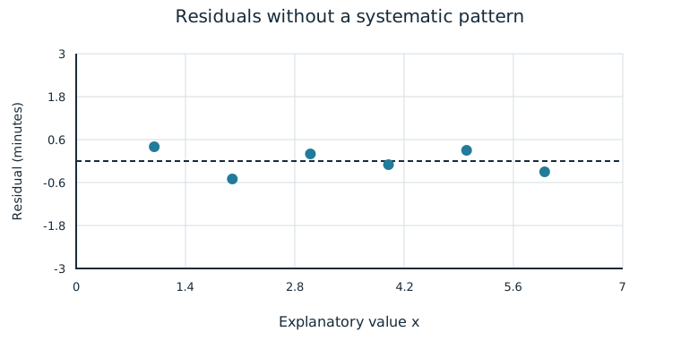
Fit a linear model when the data exhibit an approximately linear trend. Residual plots help investigate whether that form is appropriate for the observed data. If residuals scatter above and below zero without systematic shape, the plot supports a linear form. Apparent randomness is evidence for form, rather than proof that every assumption or individual prediction is correct. Look back at the original scatterplot and at the context as well.
Worked Comparison: Random Scatter or Curvature?
The first plot uses the complete residual pairs (1,0.4),(2,−0.5),(3,0.2),(4,−0.1),(5,0.3),(6,−0.3). It has no clear systematic bending across x. The second uses (1,2),(2,−1),(3,−2),(4,−2),(5,−1),(6,2). It forms a U-shaped pattern: residuals are positive at the ends and negative in the middle. The model tends to underpredict at both ends and overpredict in the middle. This curvature suggests that a linear model is not the most appropriate form for these observations.
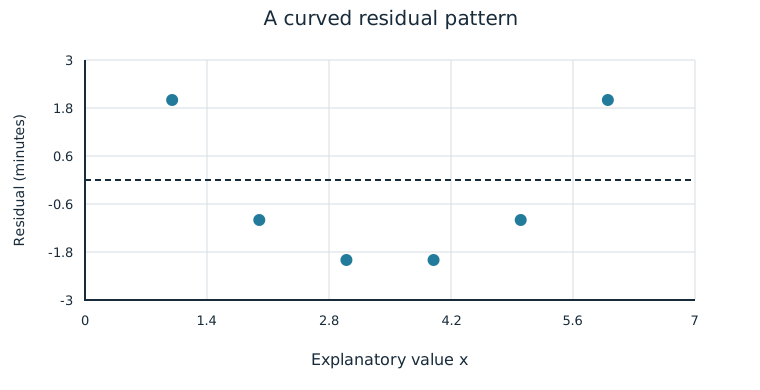
Small residuals can still follow a systematic curve; their signs and arrangement matter as well as their magnitudes. Conversely, a plot with no obvious curve can contain an unusual large residual that needs investigation. A residual plot does not authorize deleting an inconvenient observation. Describe the pattern and explain what it suggests about model form.
Worked Route Check
For the supplied model , routes at x=1,2,3 kilometers have observed times 8,8,12 minutes. Predictions are 7,9,11 minutes, giving residuals 1,−1,1 minutes. Plot (1,1),(2,−1),(3,1) against distance, or plot (7,1),(9,−1),(11,1) against predicted time. Both preserve the same residuals. Three observations alone provide little evidence about the overall form; a fuller data set can reveal a pattern that this short excerpt cannot establish.
Independent Practice
Use the information in each question to make your own calculation, representation, or argument. Explain what your result means in its setting.
Original generated practice for the Fall 2026 course.
Glossary and deeper reading · 6 refreshers
These editorial refreshers supplement the reading. Definitions and examples are added guidance; original source wording and recorded answers remain in their original context.
-
Residual
A residual is an observed response minus its predicted response. A positive residual places the observed point above the fitted line, while a negative residual places it below. For example, an observed height of 18 centimeters and a predicted height of 16 centimeters give a residual of 2 centimeters.
-
Response variable
A response variable records the outcome being studied. Its relationship to an explanatory variable can be investigated without assuming that the explanatory variable causes it. For example, plant height is a response when researchers compare fertilizer treatments.
Read more: Response variable in the captured Statistics reading →
-
Observation
An observation is a recorded value or set of values for an individual or occasion. The individual may be a person, object, or event rather than a human subject. For example, one plant’s measured height is an observation in a plant-growth study.
-
Mean
The mean is a measure of center often called an average. For a finite data set, the arithmetic mean is the sum of the values divided by their number; for a random variable, the mean is its probability-weighted expected value when that value exists. Means can be pulled toward extreme values and are not generally resistant. For example, the arithmetic mean of 2, 4, and 9 is 5.
-
Residual plot
A residual plot displays prediction residuals against explanatory values or fitted responses. Curvature can suggest that a straight-line model is inappropriate, while changing spread can challenge constant-variance assumptions. For example, a U-shaped residual pattern suggests that the line misses a curved relationship.
Read more: Residual plot in the captured Statistics reading →
-
Scatterplot
A scatterplot displays paired values of two quantitative variables as points. The horizontal coordinate represents one variable and the vertical coordinate represents the other. For example, plotting hours studied against test scores helps reveal a pattern without establishing causation.