Representing Motion
Translate among motion diagrams, equations, graph slopes, and signed graph areas.
One story, several ways to tell it
A cart starts from rest and rolls down a gentle ramp. We could describe that trip with a sentence, a row of position dots, a graph, or an equation. These aren’t separate types of physics. They’re different ways to show the same physical behavior.
A motion diagram marks positions at equal time intervals. Equal spacing means constant speed; increasing spacing means speeding up. Arrows between dots can show velocity. Don’t confuse the dots’ spacing with a position–time graph: a graph also has a time axis, and the slope carries the velocity information.
For a position–time graph, a tangent is a straight line that matches the curve’s local direction at one point; its slope gives instantaneous velocity. A secant joins two plotted points; its slope gives average velocity between them. For a velocity–time graph, tangent slope gives acceleration, while signed area gives displacement. For an acceleration–time graph, signed area gives the velocity change. Above the time axis counts positive; below counts negative. Speed and total distance use magnitudes instead.
Constant acceleration makes a useful shortcut
If acceleration is constant for an interval, velocity changes by equal amounts in equal times. The velocity graph is a straight line, so its area is a rectangle plus a triangle. That geometry gives us:
v_f = v_i + aΔt
Δx = v_iΔt + ½a(Δt)²
v_f² = v_i² + 2aΔx
The third equation comes from eliminating time from the first two. Use signed components from one consistent axis. These are equations for constant acceleration, not formulas to drop into every problem. If acceleration varies, qualitative graph reasoning still works; AP Physics 1 doesn’t require numerical analysis of nonuniform acceleration.
Example 1.3.1 — The ramp cart
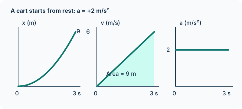
A cart has v_i = 0 and constant acceleration +2 m/s² for 3 s. The final velocity is +6 m/s. The triangular area under its velocity graph is ½(3 s)(6 m/s) = +9 m. The displacement equation gives the same result: ½(2)(3²) = 9 m.
Its position graph curves upward, starting with zero slope and growing steeper. Its velocity graph rises linearly from 0 to 6 m/s. Its acceleration graph stays flat at +2 m/s². All three graphs must agree. A straight position graph paired with that rising velocity graph would describe two different motions.
Now suppose the cart enters the ramp already moving at +1 m/s. The velocity graph starts above zero. The displacement includes a 3 m rectangle plus the 9 m triangle, giving 12 m. That rectangle is why simply using the triangle formula fails when initial velocity isn’t zero.
What happens at the top of a toss?
Near Earth’s surface, a freely moving object has downward gravitational acceleration approximately 10 m/s² when air resistance is neglected. With upward positive, a_y = −10 m/s² during the upward trip, at the highest point, and during the downward trip. Velocity at the highest point is zero for a vertical toss, but acceleration isn’t. “Not moving at this instant” does not mean “velocity is not changing.”
For a ball tossed up at 20 m/s, v = 20 − 10t, so the highest point occurs after 2 s. Its upward displacement is 20(2) − 5(2²) = 20 m. On return to the same height after 4 s, net displacement is zero while distance traveled is 40 m. Use g = 10 m/s² for our AP numerical examples; correctly using a more precise accepted g is also allowed by the supplied CED.
Make the graphs earn their keep
Use a motion sensor to record a cart speeding up approximately uniformly. Fit a straight line to velocity versus time and report its slope with units. Independently find displacement from the velocity graph’s area and compare it with measured position change. State a time interval, label scales, and use a best-fit trend rather than selecting whichever two noisy points agree with your expectation. If the acceleration graph isn’t approximately horizontal, say why the constant-acceleration equations are only an approximation.
Change it & predict
Make a motion graph
A cart starts at x = 0 with velocity +2 m/s. Keep its acceleration constant, and predict the graph before moving the controls.
The slope is acceleration. The shaded signed area is displacement; a part below zero subtracts from it. Total distance would add the magnitudes of both parts. If the line crosses zero, the cart changes direction.
Example 1.3.2 — Derive and check the three equations
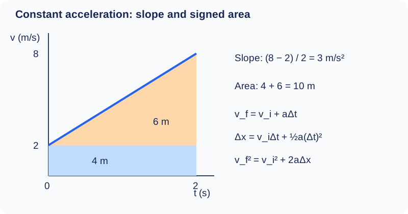
For a straight velocity–time graph, its constant slope gives a = (v_f − v_i)/Δt, so v_f = v_i + aΔt. Its signed area is a rectangle v_iΔt plus a triangle ½(aΔt)Δt, giving Δx = v_iΔt + ½a(Δt)². Equivalently the trapezoid area is Δx = ½(v_i + v_f)Δt. Multiply the latter relation by 2a and use aΔt = v_f − v_i: 2aΔx = (v_i + v_f)(v_f − v_i) = v_f² − v_i². Thus v_f² = v_i² + 2aΔx. This derivation does not require dividing by a, so it also retains the zero-acceleration case.
A cart starts at x₀ = −1 m with vₓ₀ = +2 m/s and constant aₓ = +3 m/s² for 2 s. The first equation gives vₓ = +8 m/s. The second gives x = −1 + 2(2) + ½(3)(2²) = +9 m, hence Δx = +10 m. The third independently checks 8² = 2² + 2(3)(10) = 64 m²/s². Its square alone would not determine the final velocity’s sign; the first equation and motion establish +8 m/s.
All three equations describe instantaneous endpoint quantities during one constant-acceleration interval. For nonuniform acceleration, reason qualitatively about slopes and areas instead of substituting one acceleration into these formulas. In free-fall numerical examples we use g ≈ 10 m/s²; consistent use of 9.8 or 9.81 m/s² is also accepted.
Inspect diagram labels
The diagram keeps its full size here. Focus the view and use the arrow keys, or scroll across it, to inspect every label.
Check what you know
Pause & try it
Let's see what stuck.
Choose an answer, then check the reasoning. Try the written problems below before opening their solutions.
0 of 3 checked · 0 correct
Give it a try
Practice 1
A cart’s velocity is +4 m/s for 2 s, then falls linearly to zero during the next 2 s. Sketch v versus t, and find displacement and the acceleration in each interval.
Practice 2
Derive Δx = ½(v_i + v_f)Δt from a straight velocity–time graph. State the condition needed for that graph.
Practice 3
A falling ball experiences increasing air resistance. Sketch the qualitative velocity and acceleration graphs with downward positive. Explain why a constant downward acceleration graph would fail.
Keep exploring
Use the existing Variables of Motion for additional equations and quizzes, then check every equation against the graph relationships here.
Course scope and standards: the supplied AP Physics 1 CED, printed pages 30, 31; Topic 1.3 and its exact learning objectives. The official College Board CED is the public source; the project audit records the supplied edition.
Supporting physics references: OpenStax: constant-acceleration equations; OpenStax: falling objects. These lessons, diagrams, examples, and practice questions were written for this book.
Explain and apply the model
Try these problems before opening the solutions. State your assumptions, show the diagram or calculation, and explain what makes your answer follow.
Derive and cross-check a braking model
A cart begins at x₀ = −5 m with vₓ₀ = +12 m/s. During the next 3 s its acceleration is constant at aₓ = −3 m/s². Use a single right-positive axis.
(a) Derive all three constant-acceleration equations vₓ = vₓ₀ + aₓt, x = x₀ + vₓ₀t + ½aₓt², and vₓ² = vₓ₀² + 2aₓ(x − x₀) from the slope and signed area of a velocity–time graph. Show the time elimination for the third equation and state the condition shared by the three equations.
(b) Calculate the final signed velocity and position after 3 s with the first two equations. Independently check the final velocity’s square using the third equation. Explain why taking only a square root would not fix the direction of the final velocity.
Your written working
Drawing is temporarily unavailable. Work on paper if needed, then record your reasoning here.
Saving written working requires JavaScript. The problem remains available above; keep your work on paper or in your own notes.
Glossary and deeper reading · 7 refreshers
These editorial refreshers supplement the reading. Definitions and examples are added guidance; original source wording and recorded answers remain in their original context.
-
Velocity
Velocity describes how position changes with time and includes direction. Instantaneous velocity describes one moment, while average velocity is displacement divided by elapsed time. For example, a car turning a corner can change velocity while maintaining the same speed.
-
Instantaneous velocity
Instantaneous velocity is the rate of change of position at a particular moment. On a position-versus-time graph, its component is the slope of the tangent at that time. For example, the velocity just before a ball lands differs from the average velocity of its entire flight.
-
Average velocity
Average velocity is the displacement over an interval divided by the elapsed time. It is a vector and need not equal the average speed, which uses total distance. For example, a runner who returns to the starting line has zero average velocity for the full lap.
-
Acceleration
Acceleration is the vector rate of change of velocity with time. It can change an object’s speed, direction, or both, and it is measured in meters per second squared. For example, a satellite moving at constant speed in a circular orbit accelerates toward the center.
-
Vector component
A vector component describes the part of a vector along a chosen axis. Its signed value changes when the axes change, even though the physical vector remains the same. For example, a diagonal launch velocity can be resolved into horizontal and vertical components that share the same elapsed time.
-
Drag
Drag is a force from a fluid that opposes an object’s motion relative to that fluid. Its dependence on speed, shape, and fluid properties varies with the physical regime. For example, a parachute increases air drag by presenting a large area to the moving air.
-
Displacement
Displacement is the vector change in position from the start of an interval to its end. It depends on those endpoints rather than the length or shape of the path traveled. For example, walking around a closed track and returning to the start gives zero displacement but a nonzero distance traveled.