Rotational Kinematics
Represent angular position, velocity, and acceleration with equations and graphs.
Give the turn a coordinate
We already know how to describe a cart moving along a line. Now imagine watching a marked point on a wheel. Instead of its horizontal position, track its angular position θ about a stated axis. Pick counterclockwise as positive when viewed from the front. Clockwise motion then has negative angular velocity. The viewpoint matters: the same wheel looks clockwise from one side and counterclockwise from the other.
Angular displacement is Δθ = θ_f − θ_i. Use radians: one revolution is 2π rad, and a half-turn is π rad. A wheel can finish at the same orientation after one full turn while having Δθ = 2π rad. Keep an “unwrapped” angle when following several turns rather than resetting θ to zero every revolution.
A rigid system keeps its shape as it rotates. Different points move in different directions and at different linear speeds, so replacing the whole spinning wheel with one point would hide its rotation. However, when studying a wheel’s overall travel or a planet’s orbit, an object model at the center of mass can be appropriate if the spin is irrelevant to the question. Choose the model for the motion you need to explain.
The familiar relationships, with new names
Average angular velocity is ω_avg = Δθ/Δt, in rad/s. Average angular acceleration is α_avg = Δω/Δt, in rad/s². Angular velocity tells you how fast and which way the angle changes; angular acceleration tells you how the angular velocity changes.
For constant angular acceleration, the linear kinematics equations have these rotational partners:
- ω_f = ω_i + αΔt
- Δθ = ω_iΔt + ½α(Δt)²
- ω_f² = ω_i² + 2αΔθ
- Δθ = ½(ω_i + ω_f)Δt
The last relation uses the average of the endpoints because ω changes linearly with time. Do not apply it to a curved angular-velocity graph unless you know the true average. Constant α is a model assumption, just as constant a was in linear motion.
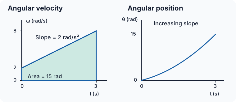
Worked example: a wheel speeds up
A wheel turns counterclockwise at 2.0 rad/s. A constant angular acceleration of +2.0 rad/s² acts for 3.0 s. Then ω_f = 2.0 + 2.0(3.0) = +8.0 rad/s, and Δθ = 2.0(3.0) + ½(2.0)(3.0²) = +15 rad. This is 15/(2π) ≈ 2.39 turns. The ω–t graph is a straight rising line. Its trapezoid area, ½(2.0 + 8.0)(3.0), gives the same 15 rad.
Now suppose the wheel initially has ω_i = −8.0 rad/s and α = +2.0 rad/s². It is rotating clockwise and slowing down. At 4.0 s it stops; after that it rotates counterclockwise and speeds up. Positive angular acceleration does not automatically mean increasing speed. Compare the signs of ω and α: matching signs increase angular speed, opposite signs decrease it.
Read all three graphs together
The slope of a θ–t graph is ω. A steepening curve means increasing angular speed in that direction; a turning point means ω = 0. The slope of an ω–t graph is α. Its signed area is Δθ, so clockwise portions subtract from counterclockwise portions. The signed area under an α–t graph is Δω. A wheel can accumulate a large total angle traveled while having small net angular displacement if it reverses.
A constant nonzero ω produces a straight θ–t graph, a horizontal ω–t graph, and an α–t line at zero. That wheel is rotating steadily, not stopped. This distinction will become rotational equilibrium later.
Instructional example (guided activity):
Video task: Put a visible mark on a slowly turning wheel and record it from directly along its axis. Record θ at equal time intervals, unwrap complete turns, and plot θ in rad against t in s. Estimate ω from neighboring slopes, then plot ω against t. State whether a constant-α model fits the data. Improve precision by using several frames per interval and avoiding a tilted camera that distorts the circle. This practices a measurable procedure and quantitative graphing.
Worked example — Use all three kinematic relationships
A rigid wheel has θ₀ = 1.0 rad, ω₀ = +2.0 rad/s, and constant α = +3.0 rad/s² for 2.0 s. Its angular velocity is ω = ω₀ + αt = +8.0 rad/s. Its angular position is θ = θ₀ + ω₀t + ½αt² = 11 rad, so Δθ = +10 rad. The time-eliminated check gives ω² = ω₀² + 2α(θ − θ₀): 64 = 4 + 2(3)(10), in consistent squared-angular-speed units. Every equation assumes the same constant angular acceleration.
The one-dimensional linear partners are v = v₀ + at, x = x₀ + v₀t + ½at², and v² = v₀² + 2a(x − x₀). The correspondence is x ↔ θ, v ↔ ω, and a ↔ α. Angular displacement, angular velocity, and angular acceleration have the same mathematical roles as the linear quantities; an ω–t line’s slope is α and its trapezoid area is Δθ.
Rigidity means the wheel holds its shape, yet points on opposite sides have oppositely directed tangential velocities. A single point at its stationary center cannot represent that spin. To describe internal rotation the extended rigid-system model is necessary. For Earth’s revolution about the Earth–Sun center of mass, an object at Earth’s center can instead describe the orbital path when its daily axial spin is irrelevant to the requested motion. This approximation discards spin details, not the orbital motion.
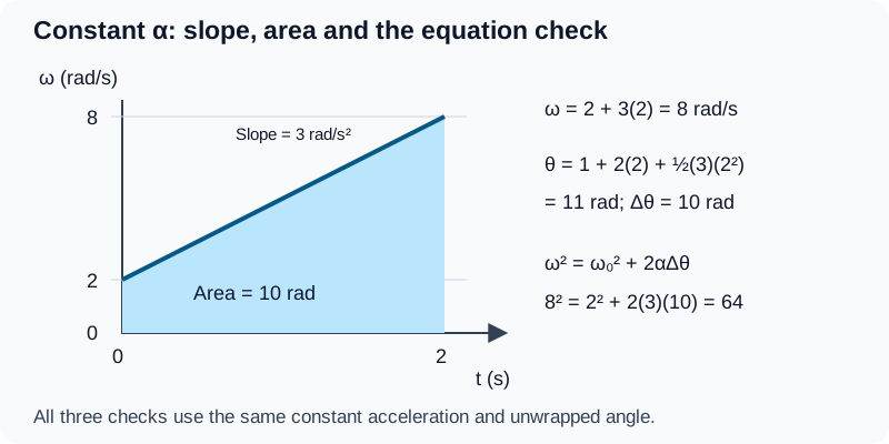
Inspect diagram labels
The diagram keeps its full size here. Focus the view and use the arrow keys, or scroll across it, to inspect every label.
Follow the turn
Pause & try it
Let's see what stuck.
Choose an answer, then check the reasoning. Try the written problems below before opening their solutions.
0 of 3 checked · 0 correct
Assigned practice: braking to rest
A wheel initially turns at +12 rad/s and comes to rest with constant α = −3.0 rad/s². Find the stopping time and angular displacement.
Open the separate worked solution.
Assigned practice: unwrap the filmed turn
A mark on a wheel has camera orientations 350°, 30°, 90°, and 170° at t = 0, 1, 2, and 3 s. It turns continuously counterclockwise and completes less than one turn between frames. Construct its unwrapped angular displacement from the first frame in radians. Use the data to decide whether constant angular acceleration is a reasonable model, and state one limitation of drawing that conclusion from only these four frames.
Open the separate worked solution.
The book’s Circular Motion and Angular Forces connect this description to the original diagrams and quizzes. Keep the new angular graphs alongside those readings.
Sources and scope: College Board CED, with edition-specific coverage verified against the supplied file. Supplied College Board CED, printed pp. 93–94, 5.1.A and the clockwise/counterclockwise boundary. OpenStax: Rotational Variables and Constant Angular Acceleration verify the variable definitions and constant-acceleration relationships. Three-dimensional angular-vector directions are enrichment, not required here.
Explain and apply the model
Try these problems before opening the solutions. State your assumptions, show the diagram or calculation, and explain what makes your answer follow.
Match models and the full equation set
A rigid wheel rotates about a fixed central axle. Its initial angle is θ₀ = 0.50 rad, its initial angular velocity is +3.0 rad/s, and its constant angular acceleration is +2.0 rad/s² for 4.0 s. Counterclockwise is positive.
(a) Calculate ω at 4.0 s using ω = ω₀ + αt, calculate θ using θ = θ₀ + ω₀t + ½αt², and independently check the result using ω² = ω₀² + 2α(θ − θ₀). Show all three calculations and state their shared domain condition.
(b) Write the linear one-dimensional counterpart of each of the three angular equations and pair angular displacement, angular velocity and angular acceleration with their linear analogues. Sketch ω versus t and use its slope and area to check α and Δθ.
(c) Explain why a spinning rigid wheel cannot be replaced by a point at its stationary center when describing the motion of opposite rim points. Contrast this with treating Earth as an object for its revolution about the Earth–Sun center of mass while ignoring daily axial spin. State what the two models preserve and omit.
Your written working
Drawing is temporarily unavailable. Work on paper if needed, then record your reasoning here.
Saving written working requires JavaScript. The problem remains available above; keep your work on paper or in your own notes.
Glossary and deeper reading · 10 refreshers
These editorial refreshers supplement the reading. Definitions and examples are added guidance; original source wording and recorded answers remain in their original context.
-
Angular velocity
Angular velocity describes the rate and direction of rotation about an axis. For a fixed axis, a signed angular velocity is measured in radians per second, while its magnitude is angular speed. For example, points on one rigid turntable share the same angular speed even though outer points have greater linear speeds.
-
Angular displacement
Angular displacement is the change in an object’s rotation angle about a specified axis. Its sign follows the chosen rotation convention, and it is commonly measured in radians. For example, a wheel can return to the same orientation after one turn while having an angular displacement of two pi radians.
-
Radian
A radian is an angle measure defined by arc length divided by radius. One complete turn is two pi radians, and angle formulas connecting linear and rotational motion use this measure. For example, an arc whose length equals the circle’s radius subtends one radian at the center.
-
Center of mass
The center of mass is the position obtained by weighting each part’s position by its mass. Its motion represents the translational motion of the whole system under the net external force. For example, adding a heavy object to one end of a light bar shifts the center of mass toward that end.
-
Angular acceleration
Angular acceleration is the rate of change of angular velocity. For a fixed axis its sign follows the chosen positive rotation direction, and its units are radians per second squared. For example, a fan speeding up has angular acceleration, whereas one turning steadily does not.
-
Kinematics
Kinematics describes motion using position, velocity, acceleration, and time without first analyzing its forces. The familiar constant-acceleration equations apply only over intervals in which that acceleration is constant. For example, a ball falling near Earth with negligible air resistance can be modeled with constant vertical acceleration.
-
Velocity
Velocity describes how position changes with time and includes direction. Instantaneous velocity describes one moment, while average velocity is displacement divided by elapsed time. For example, a car turning a corner can change velocity while maintaining the same speed.
-
Rotational equilibrium
Rotational equilibrium means the net external torque about the chosen axis is zero. A rigid body’s angular velocity then stays constant when its rotational inertia is fixed; it need not be at rest. For example, opposing torques can balance on a wheel that is already rotating steadily.
-
Acceleration
Acceleration is the vector rate of change of velocity with time. It can change an object’s speed, direction, or both, and it is measured in meters per second squared. For example, a satellite moving at constant speed in a circular orbit accelerates toward the center.
-
Vector
A vector is a quantity with a magnitude and a direction, represented by an arrow or by components along chosen axes. Vectors add by adding corresponding components rather than simply adding their magnitudes. For example, an eastward displacement followed by a northward displacement produces a resultant pointing northeast. The zero vector has zero magnitude and no unique direction.