Experiment, Explain, and Show Your Work

Let’s make the reasoning visible

You can know which equation to use and still have trouble showing why it applies. An experiment or free-response problem asks us to make that reasoning visible: choose a system, build a representation, work through the relationships, and connect a conclusion to evidence. Those are habits you can practice throughout the book, rather than save for the week before the exam.

Edition note, checked October 2, 2026: This course uses the user’s supplied AP Physics 1: Algebra-Based Course and Exam Description, cover Effective Fall 2024, updated summer 2026. Its exam table describes 42 multiple-choice questions in 85 minutes and 4 free-response questions in 95 minutes, each section worth 50%. AP Central dates this format to the May 2027 exam. Earlier exam papers can still be useful physics practice, but use the supplied edition’s timing for this course. The table and task descriptions are on CED printed pages 170–175. An allowed calculator can help, but it doesn’t replace a model or a justified claim.

Three practices, ten skills

The course outline records the exact wording of all ten skills. Here is what they look like while you’re doing a problem:

Practice	Skills	What you actually do here
Creating representations	1.A, 1.B, 1.C	Draw a labeled force diagram or energy chart; plot numerical data with scales and units; sketch a graph whose signs and extrema match the motion.
Mathematical routines	2.A, 2.B, 2.C, 2.D	Derive from a physical law; calculate with units; compare quantities at two positions; predict a factor of change using a relationship.
Scientific questioning and argumentation	3.A, 3.B, 3.C	Design a measurable procedure; make a claim using a law or model; explain how evidence supports that claim.

All three practices matter in free response. The supplied edition assesses practices 2 and 3 in multiple choice, while practice 1’s creation tasks appear in free response. Reading an existing graph and creating a new graph are different demands, so make time for both.

Experiments are part of the course

The CED requires a minimum of 25% of instructional time in hands-on laboratory work, with students keeping evidence of their work. The activities in these lessons help you plan, analyze, and discuss experiments. A website alone cannot verify that a learner has completed a classroom laboratory program. Follow your teacher’s approved laboratory arrangement; the CED also discusses supervised virtual experiences using scientist-recorded data for particular circumstances. See printed pages 6 and 140–143.

A usable procedure says what you vary, what you measure, how you measure it, and how the data answer the question. “Use a motion sensor and calculate g” leaves out the experiment. Name the measured length, define a full cycle, state how many trials you take, and explain which graph lets you infer g. Control other variables deliberately. If your claim concerns mass, don’t change both mass and spring stiffness at once.

For a small-angle pendulum, measuring a single period with a stopwatch can make reaction time a large fraction of the reading. Time 10 full cycles, repeat that timing three times, divide by 10, and compare the spread. Measure length from pivot to bob center. Use a small, similar release angle for every length and release without pushing. Plot T² versus L so the model predicts a line with slope 4π²/g. Label the axes, units, and scale; show the measured points and draw a best-fit line through the trend. Estimate slope using two well-separated points on that fitted line, not two arbitrarily selected noisy measurements.

View diagram at full size ↗

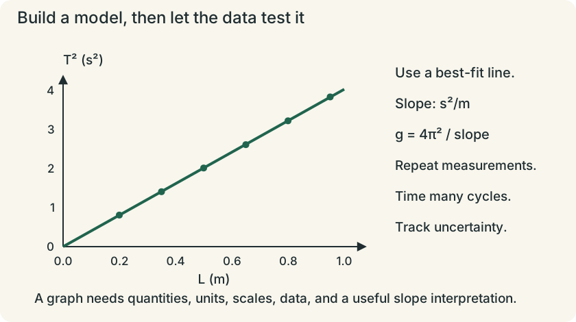
Repeats help estimate random variation. Timing more cycles reduces relative reaction-time error. Neither automatically fixes a wrongly measured pivot-to-center length or a constant sensor offset. State a specific limitation and how it affects the result. For example, a length measured consistently too short can change the graph intercept; an incorrect stopwatch time scale changes the inferred slope and g. Avoid “human error” as an explanation without saying which measurement or action matters.

The 2025 Chief Reader report reinforces the value of clear systems, energy reasoning, buoyancy force balances, measurable procedures, and useful graphs. The practice below addresses those demands with original scenarios and questions. Its teaching rubrics are ours; they aren’t official College Board scoring guidelines or a prediction of your AP score.

Let the task verb tell you what to show

Derive means start from a relevant law and show the steps to a relationship; dropping in a final formula isn’t the same thing. Calculate asks for a mathematical result with units. Compare or rank asks how quantities relate; identify what is held fixed. Justify asks for a claim supported by a physical principle or evidence, with a clear connection between them. A string of equations without that connection may leave the reader guessing.

Draw, sketch, and plot call for representations. A plot needs numerical scales and units, while a qualitative sketch still needs correct features and the labels requested. Describe asks for relevant characteristics. Determine asks for a reasoned conclusion, estimate for an approximate quantity or sign, and indicate for the requested choice. Label the specified features. Verify checks whether a definition, law, or model’s conditions hold. Read the actual request before writing a longer answer than it needs. These are paraphrased from the supplied CED’s task-verb guide, printed page 175.

Four original free-response tasks

Try each task on paper before opening its solution. The suggested times reflect the four CED task types: Mathematical Routines, Translation Between Representations, Experimental Design and Analysis, and Qualitative/Quantitative Translation. For a full timed session, fit all four into 95 minutes. Diagrams and equations below are things for you to create, not things to copy from an answer.

1. Mathematical Routines: a hanging spring

Suggested time: 20–25 minutes; teaching rubric: 10 points. A 0.30 kg mass hangs from an ideal light spring of constant 75 N/m. It settles, is pulled downward by 0.040 m from equilibrium, and is released from rest. Neglect resistance and use g = 9.8 m/s². Let x be downward displacement from equilibrium; let y be downward extension from the unstretched spring length.

1. Draw a labeled free-body diagram while x is positive. Starting from Newton’s second law and y = x + mg/k, derive aₓ in terms of x.
2. Choose a system that allows mechanical-energy conservation. Show how spring and gravitational potential combine to give an oscillation energy measured about equilibrium.
3. Derive and calculate maximum speed.
4. If the release displacement doubles with the same mass and spring, compare the period and total oscillation energy, and justify both comparisons.

Open the separate worked solution and rubric. Related instruction: restoring force, period, and vertical spring energy.

2. Translation Between Representations: a sensor’s story

Suggested time: 25–30 minutes; teaching rubric: 12 points. A 0.50 kg cart oscillates on a horizontal 50 N/m ideal spring. At t = 0 it is released from x = +0.080 m. Ignore friction.

1. Draw the cart’s horizontal force diagram at x = +A/2, then create an energy chart there showing the fractions of total energy in K and U.
2. Sketch x(t), v(t), and a(t) for one complete period on aligned time axes. Mark zero, T/4, T/2, 3T/4, and T; label extrema with the appropriate quantity and units.
3. Derive K as a function of x and sketch it from −A to +A. Calculate the total energy.
4. A second run has twice the amplitude. Describe how the time graphs and K-versus-x graph change. Explain why those changes agree with your energy equation.

Open the separate worked solution and rubric. Related instruction: reading SHM and energy.

3. Experimental Design and Analysis: find g

Suggested time: 25–30 minutes; teaching rubric: 10 points. You have a pendulum bob, string, stand, meterstick, and stopwatch. Design an experiment to estimate g using the small-angle model. State measured quantities, measurement procedures, controls, repetitions, the graph, and how its slope gives g. Give one concrete way to reduce measurement uncertainty and explain why it helps.

Another class collected the original sample data below. Each listed time is the mean elapsed time for 10 full cycles at the given length. Treat the timing uncertainty as ±0.10 s on each elapsed-time measurement and the length uncertainty as ±0.005 m.

L (m)	Time for 10 cycles (s)
0.20	8.99
0.35	11.86
0.50	14.19
0.65	16.16
0.80	17.95
0.95	19.58

Calculate the quantities for a linearized graph and plot them with scales and units. Estimate the best-fit slope and g, keeping appropriate precision. Does the evidence support g near 9.8 m/s²? Explain what a systematic measurement error could do that repeats alone wouldn’t fix.

Open the separate worked solution, graph, and rubric. Related instruction: period experiments.

4. Qualitative/Quantitative Translation: buoyancy and acceleration

Suggested time: 15–20 minutes; teaching rubric: 8 points. Two rigid sealed blocks have the same external volume V and masses m and 2m. They are both fully submerged in a stationary incompressible fluid of density ρ, with ρV = 3m. They are released from rest; drag is negligible initially, and neither touches a boundary.

1. Without equations, compare their buoyant forces and initial accelerations. Justify using displaced fluid and force balance.
2. With upward positive, derive each acceleration in terms of g.
3. Explain why saying “the heavier block has half the acceleration because the same force acts on it” fails here.
4. The blocks later float freely at rest without other vertical forces. Find each submerged volume fraction and explain how both floating states are consistent with your initial acceleration results.

Open the separate worked solution and rubric. Related instruction: density and buoyancy.

For more practice, the original book keeps 30 harmonics problems and 30 fluids problems, with their own harmonics solutions and fluids solutions. Use the AP topic labels and enrichment labels to choose the right scope.