Reading SHM: Position, Velocity, and Acceleration
Connect position, velocity, and acceleration graphs with slopes, signs, and turning points.
Three graphs, one cart
Imagine a motion sensor watching our spring cart. It gives a position graph, but the graph can tell us much more than where the cart was. Its slope tells us velocity. How that slope changes tells us acceleration. Now, connect that picture to the spring force and we have three ways to describe the same motion.
For a cart released from rest at x = +A when t = 0, one convenient model is x(t) = A cos(2πft). A is the positive amplitude, the greatest distance from equilibrium, and f is the frequency in Hz. The angle 2πft is measured in radians. When t = T = 1/f, the argument is 2π and the cart is back at +A. If the cart starts at equilibrium moving right, x(t) = A sin(2πft) is more convenient. These describe different choices of starting time, not different types of oscillator.
Read the turning points first
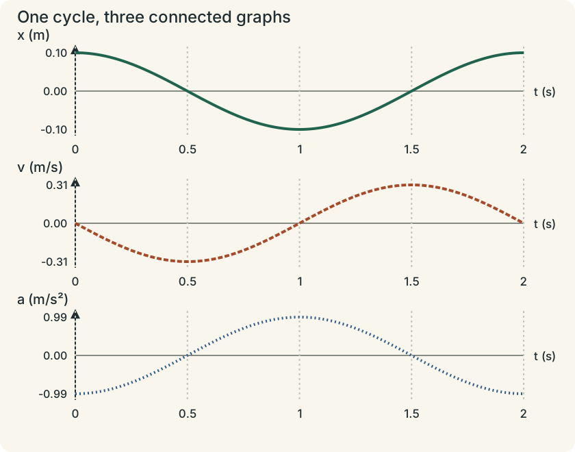
For the cosine start, at t = 0 the cart is at +A, so v = 0 and a is most negative. At t = T/4, x = 0, v is most negative, and a = 0. At t = T/2, x = −A, v = 0, and a is most positive. At t = 3T/4, x = 0 and v is most positive. At t = T, we’re back where we started. Notice that x = 0 happens twice in a cycle, with different velocity directions. Position alone doesn’t identify the whole state of motion.
Here are useful companion expressions, with angular frequency ω = 2πf:
v(t) = −Aω sin(ωt) and a(t) = −Aω² cos(ωt) = −ω²x(t).
You can read the relationships without differentiating anything. Velocity is the slope of x(t); an x maximum has a horizontal tangent and therefore zero velocity. The steepest position slope occurs at equilibrium, where speed is largest. Acceleration is the slope of v(t), and Newton’s law gives the same answer through a = −(k/m)x. Displacement and acceleration have opposite signs at every nonzero x. Velocity isn’t always opposite to acceleration: sometimes the cart is speeding up and sometimes it is slowing down. OpenStax’s SHM treatment supports these graph relationships; our graphs and tasks are original.
A worked sensor reading
Suppose the positive position peaks are 0.12 m at t = 0.30 s and again at t = 1.10 s, and the midline is x = 0. The amplitude is 0.12 m, the period is 0.80 s, and f = 1.25 Hz. Don’t call 0.24 m the amplitude: that is the full peak-to-peak displacement. Here ω = 2π/0.80 = 7.85 rad/s, so v_max = Aω = 0.942 m/s, and a_max = Aω² = 7.40 m/s². At t = 0.50 s, one quarter-cycle after the positive peak, the cart is at x = 0 moving left. Its velocity is −0.942 m/s and acceleration is zero.
What if the sensor uses a coordinate origin at the wall instead of at equilibrium? If the midline is x_sensor = 0.50 m, use x = x_sensor − 0.50 m in the restoring-force equation. The peaks at 0.62 m and 0.38 m are still 0.12 m away from equilibrium. A coordinate offset doesn’t change the amplitude or period. This is a common place for a perfectly good graph to produce a wrong force calculation.
Bigger amplitude, same time spacing
Keep the same ideal mass and spring, but double A. The position peaks become twice as high, and the velocity and acceleration extrema double too. The time between peaks stays unchanged, since T depends on m/k rather than A. On a graph, stretch the curves vertically while keeping the same horizontal scale. With fixed amplitude instead, doubling frequency doubles v_max and quadruples a_max. The units give a quick check: Aω is m/s and Aω² is m/s².
These comparisons connect the period lesson with oscillator energy: doubling amplitude doubles maximum speed, which makes maximum kinetic energy four times bigger. A larger amplitude doesn’t automatically mean a larger frequency. If a real sensor records shorter or longer periods at larger pulls, investigate the linear-force assumption before announcing that the ideal SHM model predicts it.
Try a graph before another equation
Record motion for several cycles, or use the original data below as a graph exercise. At t = 0, 0.25, 0.50, 0.75, and 1.00 s, displacement is +0.080, 0, −0.080, 0, and +0.080 m. Plot x with labeled units and a smooth curve. Sketch v below it on the same time scale, labeling its zeros and signs; then sketch a. Explain why the acceleration at 0.50 s is positive while velocity is zero. If you collect data yourself, choose a sampling interval much shorter than the period. Sparse measurements can hide extrema or make a smooth motion look jagged.
Change it & predict
Follow one whole oscillation
A 1 kg cart is on a 25 N/m spring, so ω = 5 rad/s. Start at the right turning point and follow its position, velocity and acceleration.
The curves have different units before normalization, so compare their timing, not their unscaled heights. At equilibrium, acceleration is zero and speed is greatest. At either turning point, velocity is zero and acceleration is greatest in magnitude. A bigger amplitude changes the values; it leaves this ideal period unchanged.
Choose the function from the starting state
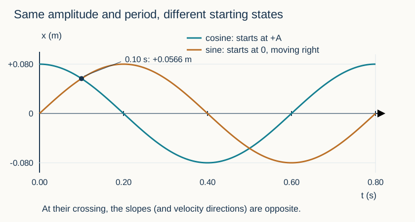
Two carts have the same amplitude 0.080 m and period 0.80 s, so both have f = 1/0.80 = 1.25 Hz. Cart C starts at its positive turning point; cart S starts at equilibrium moving right. For these choices of t = 0, write x_C = (0.080 m) cos[2π(1.25 Hz)t] and x_S = (0.080 m) sin[2π(1.25 Hz)t]. These are displacements from equilibrium. A sensor’s unrelated position offset would have to be added separately.
At t = 0.10 s, the angle is π/4 radians, so both displacements are +0.080/√2 = +0.0566 m. Equal positions do not mean equal motion: C’s position graph is falling and it moves left; S’s graph is rising and it moves right. At t = 0.20 s, the angle is π/2, giving x_C = 0 and x_S = +0.080 m. C is crossing equilibrium while S is at a turning point. You can get all these values and signs from special-angle trigonometry and graph slopes; no differentiation is required.
Inspect diagram labels
The diagram keeps its full size here. Focus the view and use the arrow keys, or scroll across it, to inspect every label.
Use a quick starting-state check before evaluating a function: cosine gives x(0) = +A, while positive sine gives x(0) = 0 with a rising graph. If the cart instead starts at equilibrium moving left, use −A sin(2πft). Changing this sign changes the initial direction, not the positive amplitude A or the frequency.
Read the motion
Pause & try it
Let's see what stuck.
Choose an answer, then check the reasoning. Try the written problems below before opening their solutions.
0 of 3 checked · 0 correct
Written practice: a graph and a symbolic comparison
A position graph has peaks +0.050 m and troughs −0.050 m, with successive positive peaks 0.40 s apart. Find its maximum speed. A second oscillator has the same amplitude and half the period. Compare their maximum accelerations.
Open the separate worked solution.
The original Simple Harmonics chapter extends sinusoidal representations to standing waves. A wave graph versus position is different from this cart’s position-versus-time graph, so always read the horizontal-axis label.
Teaching reference: CED topic 7.3, printed page 126 includes sinusoidal displacement, graph features, and amplitude changes.
Written practice: turn measured positions into a graph
A motion sensor records displacement from equilibrium for a horizontal spring cart. Its position uncertainty is approximately ±0.002 m; assume negligible friction and an ideal linear spring. Plot the measured positions below on a numerical x-versus-t graph with labeled units and scales, then sketch a smooth trend. Estimate amplitude and period from the graph and calculate maximum speed. On aligned qualitative velocity and acceleration graphs, mark the signs and important features at t = 0.20 s and t = 0.40 s. Explain whether the measured points are consistent with an SHM model, while recognizing what a short data record can establish.
| Time t (s) | Measured displacement x (m) |
|---|---|
| 0.00 | +0.081 |
| 0.10 | +0.056 |
| 0.20 | +0.001 |
| 0.30 | −0.057 |
| 0.40 | −0.079 |
| 0.50 | −0.056 |
| 0.60 | −0.001 |
| 0.70 | +0.057 |
| 0.80 | +0.080 |
Open the separate worked solution.
Explain and apply the model
Try these problems before opening the solutions. State your assumptions, show the diagram or calculation, and explain what makes your answer follow.
Choose a sinusoid from the release
Two ideal horizontal spring carts each have amplitude A = 0.060 m and period T = 1.20 s. Displacement x is measured from equilibrium, with right positive. At t = 0, cart C is released from rest at x = +A; cart S passes x = 0 moving right. Use radians in trigonometric arguments. You may use sin(π/4) = cos(π/4) = 1/√2.
(a) Calculate f, then select and write a sine or cosine displacement function x(t) for each cart. Verify each choice from its initial displacement and graph direction rather than from its name.
(b) Evaluate both functions at t = 0.15 s and t = 0.30 s. Sketch both x-versus-t curves for one period on the same labeled axes, mark those times, and explain why equal positions at 0.15 s do not imply equal velocities.
(c) A third cart has the same A and T but starts at equilibrium moving left. Write its displacement function and explain which properties change and which stay fixed.
Your written working
Drawing is temporarily unavailable. Work on paper if needed, then record your reasoning here.
Saving written working requires JavaScript. The problem remains available above; keep your work on paper or in your own notes.
Glossary and deeper reading · 11 refreshers
These editorial refreshers supplement the reading. Definitions and examples are added guidance; original source wording and recorded answers remain in their original context.
-
Velocity
Velocity describes how position changes with time and includes direction. Instantaneous velocity describes one moment, while average velocity is displacement divided by elapsed time. For example, a car turning a corner can change velocity while maintaining the same speed.
-
Acceleration
Acceleration is the vector rate of change of velocity with time. It can change an object’s speed, direction, or both, and it is measured in meters per second squared. For example, a satellite moving at constant speed in a circular orbit accelerates toward the center.
-
Amplitude
Amplitude is the maximum magnitude of a repeating disturbance measured from its equilibrium value. It describes the size of the oscillation rather than its frequency or propagation speed. For example, pulling a spring-mounted mass farther from equilibrium increases its oscillation amplitude when it is released from rest.
-
Frequency
Frequency is the number of complete repeating cycles per unit time. It is measured in hertz, meaning cycles per second, and is the reciprocal of the period. For example, a vibrating string with a higher frequency produces more cycles each second.
-
Angular frequency
Angular frequency measures how rapidly the phase of a sinusoidal oscillation advances. It equals two pi times the ordinary frequency and is measured in radians per second. For example, two oscillators at the same ordinary frequency also have the same angular frequency even if their amplitudes differ.
-
Mechanical equilibrium
Mechanical equilibrium means there is no translational or angular acceleration for the system being considered. For a rigid body, both the net external force and the net external torque must vanish. For example, a stationary ladder supported against a wall requires both force balance and torque balance.
-
Displacement
Displacement is the vector change in position from the start of an interval to its end. It depends on those endpoints rather than the length or shape of the path traveled. For example, walking around a closed track and returning to the start gives zero displacement but a nonzero distance traveled.
-
Oscillation period
An oscillation period is the time required for one complete repeating cycle. It is the reciprocal of frequency and is measured in seconds. For example, measuring the time for several pendulum swings and dividing by the number of cycles estimates the period.
-
Kinetic energy
Kinetic energy is energy associated with motion relative to a chosen reference frame. For a nonrelativistic translating object it is one half of its mass times speed squared. For example, doubling a cart’s speed quadruples its translational kinetic energy when its mass stays fixed.
-
Simple harmonic motion
Simple harmonic motion occurs when the net restoring force is proportional to displacement from equilibrium and points in the opposite direction. The resulting position varies sinusoidally with time in the ideal model. For example, a mass attached to an ideal spring can execute simple harmonic motion when damping is negligible.
-
Radian
A radian is an angle measure defined by arc length divided by radius. One complete turn is two pi radians, and angle formulas connecting linear and rotational motion use this measure. For example, an arc whose length equals the circle’s radius subtends one radian at the center.